Dynamic Potential Assessment of Source-containing Industrial Parks: A Novel Method for Sustainable Energy Grid Management
Xiaojia Sun1,*, Min Luo2, Jun Zhan1, Yuchen Lai2, Zuowei Chen1 and Tong Ye 2
1Shenzhen Power Supply Bureau Co., Ltd., Shenzhen 518001, China
2China Southern Power Grid Digital Grid Group Co., Ltd., Guangzhou 510663, China
E-mail: sunxiaojia@sz.csg.cn; 13928872104@139.com; 739564263@qq.com; laiyc@csg.cn; chenzuowei@sz.csg.cn; yetong1@csg.cn
*Corresponding Author
Received 10 November 2025; Accepted 09 December 2025
Abstract
This paper proposes a dynamic potential assessment method for source-containing industrial parks based on the Logarithmic Mean Divisia Index (LMDI) decomposition method. First, missing data are filled using Random Forest, and influence factors are quantitatively assessed by considering multi-featured factors using the LMDI decom-position method and the limit value normalization method, including distributed photovoltaic (PV) power generation impact factors, incentive tariff impact factors, energy-use behavior impact factors, and response willingness impact factors. Secondly, based on the LMDI method combined with an improved weighted polynomial regression model, the next scenario containing source industrial users is determined, providing a relatively real and reliable demand response potential assessment value. Finally, real historical response values from a certain park in the power grid were used for fitting and validation. The response deviation value was used as the evaluation criterion. Compared to the evaluation methods that do not consider data completion and those that consider only a single factor, the average response deviation rates were 4.34%, 3.23%, and 1.35%, respectively. The method proposed in this paper had the lowest average deviation rate. Additionally, this method demonstrated the changes in the weights of influencing factors. By providing a transparent and highly accurate tool for managing demand-side resources, this work facilitates greater renewable energy integration, contributing to a more efficient, stable, and sustainable power system.
Keywords: Logarithmic mean divisia index, distributed photovoltaic, source-containing industrial parks, potential assessment, demand-side response, grid sustainability.
1 Introduction
1.1 Motivation
With the large-scale integration of distributed PV power into high-penetration regional power grids, the generation and consumption uncertainties in these grids have increased. This has led to heightened challenges in regional autonomy, supply-demand interaction, and coordinated complementary dispatching. However, demand response serves as a critical strategy in the power industry to enhance the effectiveness of supply-demand interaction. It aims to improve grid stability and efficiency by incentivizing electricity consumers to increase or decrease their electricity usage during specific periods, thereby reducing reliance on expensive standby generation capacity [1]. Notably, industrial users account for more than 90% of demand-side resources [2, 3]. A significant characteristic of power systems with a high proportion of renewable energy penetration is their strong volatility [4], particularly in industrial parks with distributed PV power. These parks face significant challenges, including high generation and consumption uncertainties, potential assessments affected by time delays, and complex demand response evaluation factors.
1.2 Research Status
Current research on demand response potential assessment has actively explored various methodologies to address the aforementioned challenges [5–7]. Reference [8] uses ultra-short-term load forecasting data to cluster and depict typical user characteristics, conducting potential assessments over short periods. Reference [9] conducts a demand response potential assessment analysis on small user data and extends the mapping to derive the demand response potential assessment values for large users. Reference [10] adopts different estimation methods for different users to improve accuracy. Reference [11] quantifies the effects of cross-time period demand response using quasilinear demand response. Reference [12] comprehensively identifies, classifies, and summarizes demand response applications in the industrial sector and analyzes the complexity of industrial users’ participation in demand response. In terms of data-driven modeling, researchers have also applied advanced machine learning models. For example, Reference [13] constructed a large-scale industrial user response potential assessment model based on convolutional neural networks (CNNs), using feature selection and data reconstruction to quantify the range of adjustable loads. Reference [14] performed time series decomposition and feature extraction on industrial load data and used Gaussian process regression to assess user response potential. However, some evaluation methods also have limitations. Reference [15] employs a parameter similarity-based method for demand response potential assessment, enabling neural network training in the absence of response historical data but without fully considering individual user characteristics. References [16, 17], the authors categorize users into industrial, residential, and industrial-commercial groups. They directly process the related potential assessment data of these categories using big data methods for demand response potential analysis. However, this approach results in coarse classifications and inaccurate potential assessments. Traditional demand response potential assessment methods typically rely on simplified assumptions and historical electricity usage data, failing to intuitively present the magnitude of various influencing factors over time, nor do they provide direct references for real-time continuous peak shaving events.
When assessing the potential of short-term dynamic demand response, more factors need to be considered [18]. With the maturation of new power systems and changes in grid structure, the influencing factors and assessment scenarios for evaluating user operation potential are becoming increasingly complex [19, 20]. Against this backdrop, some studies have begun to consider the combined effects of multiple factors. Reference [21] employed the Logarithmic Mean Divisia Index (LMDI) decomposition method to analyze the energy consumption behavior and electricity prediction of users in a specific area of Shaanxi, considering multiple influencing factors. The LMDI decomposition method, with its advantage of no residual, can dynamically analyze the impact of various influencing factors on the assessment results, and has been applied in the fields of carbon emission assessment and load forecasting. Reference [22] considered the types and characteristics of industrial user equipment and conducted a cost-based demand response potential assessment analysis. Reference [23] established a closed-loop demand response potential assessment strategy in the cloud, taking into account the impact of price factors. Reference [24] considered the reducibility of air conditioning and established a hierarchical decomposition demand response potential assessment model. However, existing studies have not considered the uncertainty of distributed PV power generation, ignoring the randomness of power generation and consumption by industrial users with a high proportion of distributed PV, which can affect the accuracy of potential assessments during continuous peak regulation. At the same time, considering issues of model adaptability and computational dimensions, few studies have comprehensively considered multiple factors under different scenarios.
Table 1 Comparison of the proposed method with previous methods
| Comparison | Data-Driven | Traditional Static | |
| Dimension | Proposed Method | Assessment Methods | Assessment Methods |
| Core Methodology | LMDI for factor decomposition combined with a weighted polynomial regression model. | Utilizes various machine learning models such as CNNs, Gaussian Process Regression, or clustering algorithms. | Based on simplified physical or economic assumptions, historical electricity usage data, and static analysis. |
| Handling of PV Uncertainty | Explicitly modeled as a key dynamic influencing factor. | Generally not isolated as a distinct factor. | Typically ignored or oversimplified. |
| Consideration of Factors | Quantifies the individual contribution of multiple dynamic factors without residual error. | It is difficult to intuitively present the magnitude of various influencing factors. | Typically relies on a single dominant factor. |
| Assessment Time-Scale | Provides dynamic, short-term assessments with rolling updates to reflect real-time conditions. | Can be short-term, but models are often trained on historical data and may not adapt as dynamically. | Primarily static, long-term, or day-ahead assessments that do not capture intraday dynamics. |
| Data Handling | Employs Random Forest for data imputation, enhancing model reliability and applicability when data is missing. | Performance can be sensitive to the quality and completeness of large historical training datasets. | Highly dependent on the availability of consistent and complete historical data. |
| Key Innovation | Achieves high accuracy by quantifying and visualizing the impact of multiple uncertainties and provides an adaptable framework for dynamic potential assessment. | Capable of learning complex, non-linear relationships directly from raw data without explicit modeling. | Simplicity and ease of implementation. |
| Primary Limitation | Higher computational complexity and reliance on diverse real-time data streams. | The “black box” nature can limit interpretability and trust; models can result in coarse classifications. | Low accuracy and inability to adapt to the dynamic and complex nature of modern power systems. |
In summary, under the complex new power system for the distributed PV industrial parks with a high proportion of distributed PV, the static potential assessment in the past few days has been biased, and how to make a relatively realistic potential assessment under multiple scenarios, taking into account the uncertainty of power generation and consumption in the source-containing industrial parks and changes in the number of equipment starts and stops in the intraday dynamics, has become an urgent problem to be solved. In this paper, based on the Cloud Edge Collaboration Architecture, we use the LMDI decomposition method to analyze multiple influencing factors under multiple scenarios quantitatively, update the elasticity coefficients of the influencing factors on a rolling basis, and combine the polynomial regression method to obtain the relatively real potential assessment value of the source-containing industrial users dynamically updated within a short period. The comparison of the proposed method with previous methods is shown in Table 1.
1.3 Paper Organization
In the context of a complex new power system, this paper addresses the issues of increased uncertainty in power generation and consumption in industrial parks with a high proportion of distributed PV and the susceptibility of potential assessments to time delays during actual grid operation. A weighted polynomial regression model based on the LMDI decomposition method without residues is proposed. This method, based on a cloud-edge collaborative architecture, uses the LMDI decomposition method to normalize and analyze multiple influencing factors under various scenarios. By rolling updates of the elasticity coefficients of the influencing factors and combining them with polynomial regression, it obtains a relatively true potential assessment value for industrial users with sources, updated dynamically within a short period. Thus, this method can, under multiple scenarios, comprehensively consider various influencing factors and demonstrate the dynamic changes in their weights, enhancing the authenticity and intuitiveness of the potential assessment. The main innovations of this paper are reflected as follows:
(1) Using Random Forest data complementation combined with the LMDI decomposition method, we can simultaneously normalize and quantify multiple influencing factors under multiple scenarios, including distributed PV power generation, incentive tariff, energy-use behavior, and response willingness, to make the potential assessment data more reliable.
(2) The use of LMDI residual-free decomposition of factors affecting potential assessment facilitates the addition or reduction of missing influencing conditions, and paired with Random Forest Data Completion, it can lead to a significant increase in model adaptation within limited data. At the same time, it can visualize the size of the influence factor over time, which can intuitively reflect the influence factors of potential assessments in different time periods.
(3) Based on the cloud-side synergistic potential assessment framework, the impact of distributed PV capacity and generation uncertainty is added to the assessment model, which can make a dynamic, short-term, and relatively accurate assessment of industrial users containing distributed PV through the rolling update of quantitative factors.
The remainder of this paper is organized as follows: Section 2 introduces the cloud-edge collaborative potential assessment framework. Section 3 constructs the multi-factor LMDI decomposition model and data completion method. Section 4 proposes the improved weighted polynomial regression model for dynamic assessment. Section 5 presents the case study analysis and method comparison. Finally, Section 6 concludes the paper.
2 A Framework for Assessing the Cloud Edge Potential of Source-containing Industrial Parks
Demand response potential assessment for users in source-containing industrial parks is characterized by rapid changes in distributed power generation data, the coupling of factors influencing electricity consumption behavior, incentive prices, and response willingness, which presents significant challenges to actual power system dispatch. Nowadays, the widespread adoption of 5G signals, the maturation of data cloud systems, and the increasing sophistication of smart terminals enable the collection of more user data [25, 26].
This paper proposes a demand response potential assessment architecture nested in a cloud-edge architecture. Defining variable data is collected at the edge end, and it is easy to add or delete the collected influencing factor data because the factor screening model used is the LMDI residual-free factor decomposition method. Meanwhile, magnitude normalization and data complementation are performed at the edge end, and the corrected impact factor data are uploaded to the cloud. The potential assessment system in the cloud performs LMDI factor decomposition on the collected data and displays the weights and sizes of the impact factors in hourly rolling updates, which is convenient for providing intuitive impact factor references to management personnel when different demand response events occur. The overall framework schematic is shown in Figure 1. The overall framework consists of a cloud layer, the immediate layer of the grid that can oversee edge-end data and make potential assessments. The edge layer is the aggregator where the intelligent edge is located. The end-end layer collects data from users in industrial parks containing distributed PV.
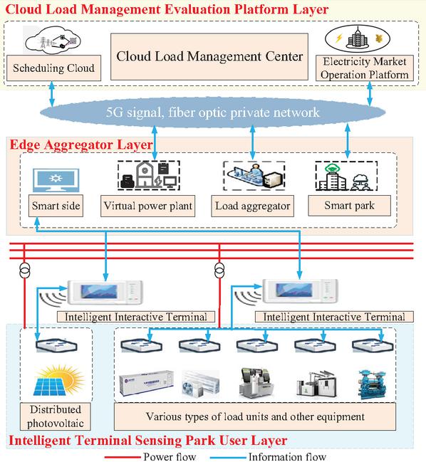
Figure 1 Schematic diagram of the cloud-edge potential assessment framework.
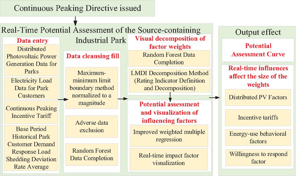
Figure 2 Overall business process diagram.
The effective operation of the proposed cloud–edge collaborative framework relies on the deployment of advanced data acquisition infrastructure, such as smart meters and 5G communication networks within the industrial park. This infrastructure forms the practical foundation for enabling high-frequency dynamic assessments.
When even the higher-level grid gives continuous peaking instructions, this model is operated to input real-time data and selected historical data of the base period within three years to assess the demand response potential of the users of the industrial park containing sources for continuous peaking from the influence factors of distributed PV power generation, incentive tariffs, energy-use behaviors, and willingness to respond, and to show the impacts of different influences on the assessed value of the potential It also shows the effect of different influencing factors on the potential assessment value, so that the dispatchers can only refer to it and make further orders and judgments. The overall business process is shown in Figure 2.
3 Multi-factor Selection and LMDI Decomposition Model Construction
To address the evaluation challenges posed by the interplay of multiple dynamic factors, including the uncertainty of distributed PV generation, incentive-based electricity pricing, user energy consumption patterns, and response willingness, this paper proposes a multitier analytical framework. The primary objective of the framework is to clearly and precisely quantify the contribution of each influencing factor, thereby enabling accurate prediction of demand response potential.
The LMDI decomposition method is well-suited for this task owing to two distinct advantages. First, it achieves a fully residual-free decomposition, attributing the entire variation in response potential exclusively to the sum of contributions from the predefined factors. This feature ensures analytical transparency and precision, while enabling system operators to directly assess the influence of each factor on the evaluation outcome, thereby supporting evidence-based decision-making. Second, the method offers high adaptability, permitting the straightforward inclusion or removal of influencing factors in response to actual data availability, an essential capability for handling complex, variable real-world data environments.
Moreover, given the prevalence of missing data in practical data acquisition, this study employs the random forest algorithm to impute incomplete historical records. This approach ensures the completeness and reliability of the dataset, forming a robust foundation for subsequent decomposition and evaluation.
The remainder of this chapter elaborates on the formulation of the influencing factor model, the data imputation methodology, and the construction process of the LMDI-based factor decomposition model.
3.1 Impact Factor Model Definition and Data Completion
The paper utilizes the LMDI residual-free factor decomposition method to simultaneously consider multiple influencing factors, including distributed PV impacts, incentive tariff impacts, energy-use behavior impacts, and user response willingness, to improve the accuracy of potential assessment. Due to the multiple considerations of the LMDI decomposition method, the influencing factors can be flexibly increased or decreased. With the use of the random forest algorithm in python to complement the data [27–28], the data can be changed flexibly in the case of missing or incomplete data, and still make a relatively accurate and reliable assessment of the response potential.
At the same time, the missing factors can be added or deleted to enhance the adaptability of the model in the limited data conditions, to make a relatively accurate and reliable assessment of the potential, and visualize the impact of the influence of the factors over time changes in the influence of the weight, can be for the management of real-time occurrence of the demand response event factors to provide a direct reference.
This paper models the four core influencing factors identified above. We acknowledge that actual demand response potential may also be shaped by additional variables, including weather conditions (which directly affect photovoltaic output), the park’s dominant industrial type (which influences load rigidity), and macroeconomic conditions. Integrating such factors into the model constitutes an important direction for future enhancement; however, to preserve the present study’s focus, these aspects are not explored herein.
3.2 LMDI-based Modeling of Impact Factor Disassembly
The LMDI decomposition method allows for a completely residual-free exponential decomposition, which separately reflects the impact of changes in each influencing factor on changes in response potential, increasing the accuracy of potential assessment while giving dispatchers an intuitive way to provide the magnitude of the factors that influence the potential assessment when continuous peaking is performed, so that the dispatchers can make reasonable judgments and adjust measures. The average value of the deviation rate of distributed PV generation, demand response incentive tariff, real-time user load, and historical demand response load shedding of plants in the park is determined as the model data input. The steps to quantify the impact factors of the LMDI decomposition method are as follows:
(1) Determine the decomposition structure
I. Define variables: Define the -th user -th hour, demand response potential ; distributed PV generation ; demand response incentive tariff ; user plant history of user demand response load shedding amount of the deviation rate of the average value .
II. Selecting the Base Period and Reporting Period: Determine the time frame of the analysis for the historical three-year assessment of industrial user demand response data, the selected year of the beginning of the data for the base year, the first response data of the base year for the base value , the rest of the analysis period data for the report year, the report year data for the report data.
(2) Data collection and pre-processing
I. Collect the data of defined variables for three years of history.
II. Data preprocessing based on the minimum-maximum limit boundaries to establish the sample data matrix set:
Scale the defined variable data for each analysis into so that all variables are in the same magnitude:
| (1) |
where is original data; and are the maximum and minimum values in the data set; is normalized data.
(3) Construct the LMDI decomposition model of the influencing factors of industrial users’ potential assessment with multi-featured factors, analyze and obtain the values of industrial users’ demand response potential assessment and the values of the elasticity coefficients of the influencing factors under different scenarios, and the model formulas are as follows:
| (2) |
where is the -th customer -th hour demand response potential assessment value; is the -th customer -th hour distributed PV generation; is the -th customer -th hour demand response incentive price; is the -th customer -th hour load. is the average value of the deviation rate of the historical user demand response load shedding for the -th customer -th hour ago.
Define the influencing factor variables as follows, is the ratio of demand response potential to distributed PV generation for the -th user at -th hour, which is defined as the distributed PV impact factor indicator; is the ratio of distributed PV generation to the demand response incentive tariff at -th hour for the -th customer, which is defined as the incentive tariff factor impact indicator; is the ratio of the demand response incentive tariff to the customer’s electricity load at -th hour for the -th customer, which is defined as an indicator of the factors influencing energy use behavior; is the ratio of the deviation rate average of the customer’s electricity load to the customer plant’s historical customer demand response load shedding at -th hour for the -th customer, which is defined as an indicator of the factors influencing the willingness to respond.
Further decomposition formula is:
| (3) |
where, , indicates the degree of contribution of each factor to the amount of change in the potential assessment from the baseline hour to the target hour, respectively, and the main factors are distributed PV power generation influencing factors, incentive tariff influencing factors, energy-use behavior influencing factors and response willingness influencing factors, respectively.
The change amount of each influence factor is:
| (4) | |
| (5) | |
| (6) | |
| (7) | |
| (8) |
where is the logarithmic mean.
4 Improved Weighted Multiple Regression Model Based on LMDI and Its Solution
The proposed approach combines multiple techniques, include random forest imputation, LMDI factor decomposition, and weighted polynomial regression, yielding a computationally intensive process. This design reflects a deliberate trade-off between computational efficiency and assessment accuracy, with the objective of capturing the influence of diverse dynamic factors to enable high-fidelity potential evaluation. The subsequent sections detail the solution workflow of this high-precision model.
4.1 Improved Weighted Multiple Regression Model for LMDI
The influencing factor sizes from the residual-free factor decomposition calculated in the LMDI decomposition method of Section 2.2 are normalized and polynomial-weighted regression is performed to obtain the potential assessment value for the next hour. Then, based on the new potential assessment value, the influencing factor weights are calculated in the base period historical data using the LMDI decomposition model of Section 2.2, and the weighted polynomial regression is repeated to calculate the latest response potential assessment value and the proportion size of the influencing factors in the next hour, and the overall framework of the model is shown in Figure 3.
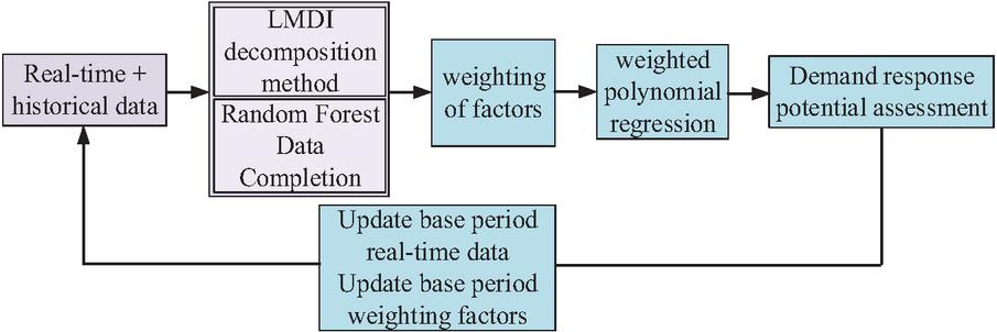
Figure 3 Improved weighted multiple regression process framework diagram based on LMDI.
The overall weighted polynomial regression model based on LMDI factor decomposition and steps is as follows:
(1) Obtain the weights and sizes of the nonresidual impact factors of the impact factors in Section 2.2, the impact ratio of the distributed PV influence factor indicator is , the impact ratio of the incentive electricity price factor indicator is , the impact ratio of the energy consumption behaviour influence factor indicator is , and the impact ratio of the response willingness influence factor indicator is .
(2) Weight the original data according to the weights.
| (9) | ||
| (10) | ||
| (11) | ||
| (12) |
(3) Standardized data to improve prediction accuracy [29].
| (13) |
where represents data on the four impact factors; and are the mean and standard deviation of , respectively.
(4) Polynomial feature expansion
The weighted features after normalization in step 3 are extended to polynomial features, including quadratic and cross terms, as in the form of (14).
| (14) |
(5) Develop a polynomial regression model to predict the assessed value of hourly park potential .
| (15) |
where is the vector of regression model coefficients; is the error adjustment term.
4.2 Model Solution and Flowchart
Firstly, ‘Simple Imputer’ and ‘Random Forest Regressor’ from Python ‘sklearn’ were utilized Random Forest Regressor’ method in python ‘sklearn,’ the historical data were supplemented, and the historical response data were factorized by combining with the LMDI decomposition model to analyze and obtain the influence ratio of the four influencing factors of fixation. Afterward, the influence factor share is brought into the standardization to get the th-order polynomial formula ((5)), where is the coefficient vector, and the prediction curve of the weighted polynomial regression should be as close as possible to the actual curve to minimize the residuals at all points, and the residual formula is:
| (16) |
In order to obtain the load condition , it is necessary to minimize the sum of squares of the residuals, i.e.:
| (17) |
Obtained by taking a partial derivative of the right-hand side of Equation (17):
| (18) |
Which is then transformed into matrix form:
| (19) |
Equation (19) is expressed in matrix form as:
| (28) | ||
| (33) |
This Vandermonde matrix is further reduced to:
| (34) |
Using Python ‘StandardScaler’ and other tools for solving, solving that is the specific model of the potential assessment curve to complete the response potential assessment prediction, the overall flowchart is shown in Figure 4. The process is divided into four main steps (Step 1 to Step 4), illustrating the clear logical flow from data input, factor decomposition, weight calculation, to the final potential assessment.
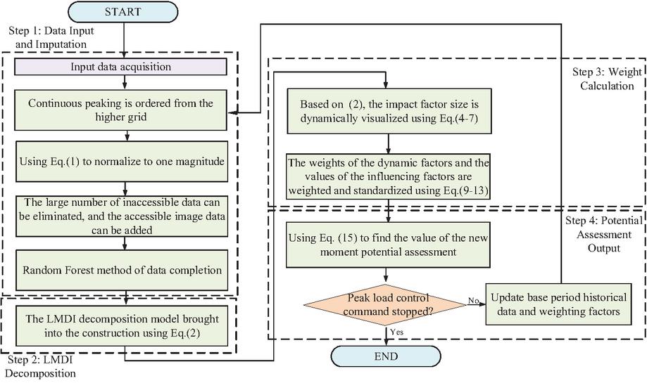
Figure 4 Flowchart of short-term dynamic potential evaluation based on LMDI decomposition method.
5 Example Analysis
5.1 Data Selection and LMDI Factor Decomposition Results
To verify the effectiveness of the proposed method, this paper selects the real operational records of a demonstration industrial park located in northern China as the dataset. This industrial park hosts 42 large-scale industrial users and operates a 75.6 MW distributed PV system. The park has significant intraday load fluctuations and participates in incentive-based demand response programs on a regular basis.
The baseline data are selected from a certain day’s continuous intraday peak-shaving load curve in the industrial park, from which the following can be obtained: the load forecast values (load curve without peak shaving), the actual demand response values (post-response curve), the expected demand response values, the PV generation data, and the intraday incentive electricity prices for demand response. The original data used in the case study are shown in Figures 5 and 6 Furthermore, the historical average deviation rate of user load reduction due to demand response over the past three months is found to be 17.3%.
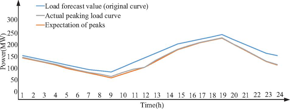
Figure 5 Load data curves comparing load forecast versus actual response values.
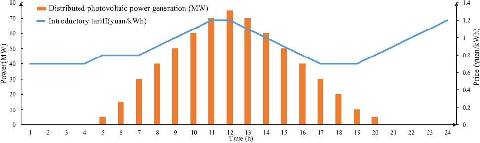
Figure 6 Data curves for intraday distributed PV power generation and demand response incentive electricity prices.
The original data is brought into the model solution to obtain the change in the proportion of the influence factor indicators, as shown in Table 2; using the LMDI decomposition method, it can be visualized that the influence factor indicators change over time in the proportion of the influence weight. The analysis can be concluded that the distributed PV power generation factor, the impact of load shedding on the assessment of demand response potential is positive and the largest impact of 78.23%, followed by the incentive tariff factor of 32.66%; energy use behavior and response willingness factors, the effect of load shedding value on the assessment of demand response potential is negative.
Table 2 Change in the contribution proportion of influencing factor indicators
| Hour | Distributed PV Factors | Incentive Tariff Factors | Energy-use Behavioral Factors | Willingness to Respond Factor | Add up the Total |
| 1 | -1.2546 | -0.2636 | 0.3737 | -1.9779 | -3.1224 |
| 2 | 4.5071 | 1.7111 | -2.5212 | 1.2618 | 4.9589 |
| 3 | 2.3199 | -1.8020 | 3.7567 | 0.8274 | 5.1021 |
| 4 | 0.9866 | 0.0854 | 2.2011 | 0.9160 | 4.1891 |
| 5 | -3.4398 | 0.5545 | 3.5160 | 1.0851 | 1.7157 |
| 6 | -3.4401 | -2.7213 | 3.1586 | -1.7038 | -4.7066 |
| 7 | -4.4192 | 0.6453 | 0.7832 | -0.5661 | -3.5568 |
| 8 | 3.6618 | -1.9769 | 3.3750 | -1.5365 | 3.5234 |
| 9 | 1.0112 | -2.6097 | -3.2921 | 1.4521 | -3.4382 |
| 10 | 2.0807 | 2.6933 | -2.4321 | 0.4932 | 2.8351 |
| 11 | -4.7942 | 2.7938 | -3.6382 | -0.6764 | -6.3150 |
| 12 | 4.6991 | 1.8504 | -1.3974 | -1.7458 | 3.4064 |
| 13 | 3.3244 | -1.1723 | -0.8906 | -0.7561 | 0.5055 |
| 14 | -2.8766 | -2.4140 | -1.8292 | -0.6993 | -7.8191 |
| 15 | -3.1818 | 1.1054 | 2.6299 | 0.9184 | 1.4720 |
| 16 | -3.1660 | -0.3591 | -1.1460 | 0.5502 | -4.1208 |
| 17 | -1.9576 | -2.2678 | -1.7525 | 1.5489 | -4.4290 |
| 18 | 0.2467 | -0.0289 | 0.3416 | -0.1111 | 0.4491 |
| 19 | -0.6806 | -2.7937 | -2.8726 | -1.5216 | -7.8684 |
| 20 | -2.0877 | 2.4559 | 2.4176 | 0.8530 | 3.6388 |
| 21 | 1.1185 | -1.4473 | -3.4036 | 1.0431 | -2.6892 |
| 22 | -3.6051 | 0.9751 | 3.8951 | 0.2451 | 1.5103 |
| 23 | -2.0786 | -1.1297 | 2.1780 | 1.0839 | 0.0535 |
| 24 | -1.3364 | 0.1204 | -2.4103 | -0.0248 | -3.6511 |
| Total | -14.3610 | -5.9956 | 1.0407 | 0.9591 | -18.3572 |
| Weight % | 78.23 | 32.66 | -5.67 | -5.22 | 100 |
To more intuitively present the dynamic changes of these factors, their contribution values are plotted in Figure 7. The figure clearly shows that the distributed PV generation factor and the energy behavior factor have large fluctuation ranges, whereas the incentive price factor and response willingness factor remain relatively stable.
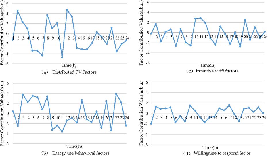
Figure 7 Fluctuation values of influencing factors of LMDI decomposition.
To further investigate the model’s sensitivity to key input variables, this study conducts a single-factor sensitivity analysis on two core variables: the incentive tariff and the photovoltaic (PV) output prediction deviation. In this analysis, other input conditions are held constant at their baseline values while a specific variable is varied within a defined range (e.g., 20%) to observe its impact on the final demand response potential assessment value. The results are presented in Figure 8.
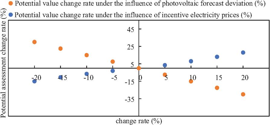
Figure 8 Sensitivity analysis of key input variables.
As shown in Figure 8, the potential assessment value exhibits a significant non-linear positive correlation with the incentive tariff. A higher price incentive leads to greater exploitable response potential, and the rate of increase accelerates as the tariff rises, indicating that the price lever is a key driving force for encouraging user participation in demand response. Conversely, the potential assessment value has a negative correlation with deviations in the PV power output prediction. Specifically, if the actual PV output exceeds the forecast (a positive deviation), the net load is lower than anticipated, and consequently, the available curtailable potential decreases, and vice versa.
5.2 Comparative Results of Fitting Different Strategies for Potential Assessment
The weighted and normalized proportions of the decomposed influencing factors in Section 4.1 were used, and nonlinear weighted polynomial regression was applied to roll predict the 24-hour demand response potential assessment results. At the same time, the potential assessment values from traditional invitation-based methods and data-mechanism hybrid methods (as described in the comparison schemes set up in this paper, see Table 3) were compared. These three schemes were selected because they represent the three major categories of existing potential assessment approaches: (1) traditional rule-based invited assessments, (2) hybrid data-driven methods widely used in industry, and (3) our proposed mechanism-driven dynamic assessment method. Together, they provide a comprehensive and fair comparison baseline. The comparison chart of the potential assessment values from different schemes is shown in Figure 9.
Table 3 Comparison scheme description
| Scheme | Description |
| Traditional solicited assessments | Following the traditional invitation-based method, only the single factor of user energy consumption behaviour is considered when estimating demand response potential. |
| Mixed data-mechanism assessment | The estimated demand response potential was calculated using a static transfer learning algorithm model. |
| Methodological assessment of this paper | The estimated demand response potential obtained by using the LMDI decomposition method and multiple regression model, considering factors such as user energy consumption behavior and the uncertainties in distributed PV generation and consumption. |
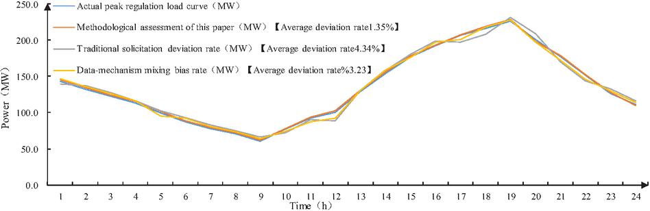
Figure 9 Comparison chart of the potential assessment values of different scenarios.
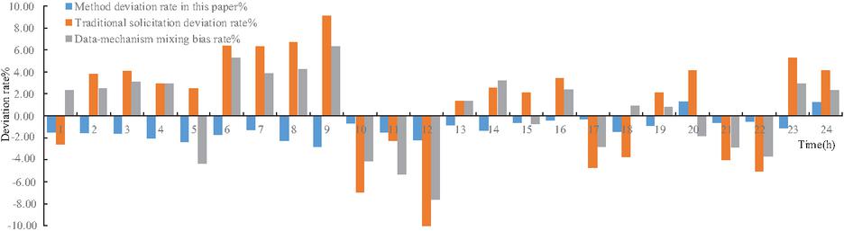
Figure 10 Exploded view of the response bias rate for different scenarios.
In order to reflect the effect of program comparison, the response deviation rate of different programs is decomposed, and the decomposition diagram is shown in Figure 10. For the source-containing industrial parks, the potential to assess the impact of the factors of the proportion of the size of the visual display of the demand for continuous peaking, so as to facilitate the controllers in making further instructions to make judgments.
Comprehensive comparison of the mean value of the absolute value of the assessment deviation rate of each scheme, the mean value of the absolute value of the deviation rate of the traditional invited assessment is 4.34%, the mean value of the absolute value of the deviation rate of the hybrid data-mechanism potential assessment is 3.23%, and the mean value of the absolute value of the deviation rate of the assessment method of this paper is 1.35%. After the overall comparison, it reflects the accuracy of the methodology, for industrial parks containing distributed power sources, for the assessment of demand response potential in the case of limited data factors, and takes into account the distributed PV generation factor, the incentive tariff factor, the user’s energy behavior factor and the willingness to respond factor.
5.3 Discussion on Model Generalizability
The case study in this paper is based on a specific industrial park. While the validation results are promising, the model’s generalizability warrants further examination. Conceptually, the proposed framework exhibits strong portability. For parks with varying industrial compositions, load profiles, or PV penetration levels, the model can be retrained on location-specific historical data to recalibrate the baseline weights and regression coefficients of each influencing factor. For instance, in heavy industrial parks characterized by continuous production, the weight assigned to behavioral energy-use factors may be lower, whereas in parks with exceptionally high PV penetration, the weight of distributed PV factors would increase substantially. Future work will involve empirical validation across diverse industrial park types to rigorously assess the model’s capacity for generalization.
6 Conclusions
For industrial parks with a high proportion of distributed PV, there is an increase in the uncertainty of power generation and consumption, data missing issues are common, actual grid operations are susceptible to time delays, and the number and complexity of factors affecting demand response potential assessments have increased. This paper proposes a short-term dynamic potential assessment method for industrial parks with high PV penetration based on the LMDI decomposition method. By combining random forest data imputation with the LMDI decomposition method without residues, this method facilitates the addition or removal of data factors, enhancing its adaptability. The influence factors obtained from the LMDI decomposition method are standardized and weighted by polynomial regression to derive the potential assessment value. Through theoretical research and simulation verification, the following conclusions were drawn:
(1) Among the influencing factors analyzed in this paper, distributed PV power generation factors and energy use behavior factors have a greater impact, and incentive tariff factors and response willingness factors have a smaller impact.
(2) Distributed PV and tariff incentive factors have a positive impact on the potential assessment, with an impact factor share of 78.23% and 32.66%, respectively. The energy use behavior and response willingness factors have a negative impact on the demand response potential assessment, with an impact factor percentage of 5.67% and 5.22%, respectively.
(3) In this paper, the potential assessment method compares the traditional invited demand response potential assessment method and the demand response potential assessment method with mixed data mechanisms, and the mean of the absolute value of the deviation rate is 4.34%, 3.23% and 1.35%, respectively.
The core contribution of this research is its role as a key technical enabler for the sustainable transition of the energy system. By significantly enhancing the assessment accuracy of demand response potential in scenarios with high PV penetration, the proposed method effectively mitigates the operational risks and uncertainties arising from the intermittency of renewable energy. This, in turn, enables the power grid to accommodate and integrate larger scales of clean energy like PV with greater confidence, directly promoting the displacement of fossil fuels. It therefore lays a solid technical foundation for achieving carbon reduction targets in the energy sector and for building a sustainable energy system for the future.
While this paper presents a dynamic evaluation approach with promising accuracy, we acknowledge several limitations that merit further investigation:
(1) Practicality and Generalizability. The proposed approach integrates multiple models, resulting in a relatively complex computational process and placing certain demands on implementers’ technical expertise and computational resources. Future work could investigate the development of a “lightweight” or simplified version, such as substituting polynomial regression with linear regression where the accuracy impact is manageable, or reducing feature dimensionality to lower model complexity. Such efforts aim to balance accuracy and computational cost, thereby reducing adoption barriers and enabling broader uptake, particularly among small-scale aggregators and utility companies.
(2) Scalability and Model Enrichment. The present study considers four core influencing factors; however, demand response potential in practice is shaped by additional variables. Future models could integrate more diverse inputs, for example: incorporating weather forecasts to improve PV output prediction accuracy; accounting for industry-specific process flows and equipment startup/shutdown costs; and including macroeconomic indicators and relevant regulatory policies. Such extensions would enhance the comprehensiveness and precision of potential assessments.
Author Contributions
Methodology, Jun Zhang, Min Luo, Yuchen Lai; software, Xiaojia Sun; validation, Tong Ye; writing-original draft, Jun Zhang, Yuchen Lai; conceptualization, Jun Zhang; reviewing and editing, Min Luo, Xiaojia Sun, Zuowei Chen; data curation, Zuowei Chen; visualization, Xiaojia Sun.
Funding
This work was supported by the Shenzhen Power Supply Bureau Co., Ltd. Technology Project: “Research and Application of Regional Large-Scale User-Side Resource Coordination and Interaction Technology” (090000KC22120002).
Data Availability Statement
The authors do not have permission to share data.
Conflicts of Interest
The authors declare no conflicts of interest.
References
[1] Wen Xu, Yang Ke, Mao Rui, et al. ‘Research and Application of Industry Standard for Evaluation of Adjustable Load Control Capacity’. Power System Technology, 45(11): 4585–4594, 2021.
[2] Xu Zheng, Sun Hongbin, Guo Qinglai. ‘Review and Prospect of Integrated Demand Response’. Proceedings of the CSEE, 38(24): 7194–7205+7446, 2018.
[3] Wang Caixia, Shi Zhiyong, Liang Zhifeng, et al. ‘Key Technologies and Prospects of Demand-side Resource Utilization for Power Systems Dominated by Renewable Energy’. Automation of Electric Power Systems, 45(16): 37–48, 2021.
[4] Ju Ping, Jiang Tingyu, Huang Hua. ‘Brief Discussion on the “Three-self” Nature of the New Power system’. Proceedings of the CSEE, 43(07): 2598–2608, 2023.
[5] Fotopoulou, M., Tsekouras, G.J., Vlachos, A., Rakopoulos, D., Chatzigeorgiou, I.M., Kanellos, F.D., Kontargyri, V. ‘Day Ahead Operation Cost Optimization for Energy Communities’. Energies, 18, 1101, 2025.
[6] Libra, Martin, Kozelka, Martin, Šafránková, Jana, Belza, Radek, Poulek, Vladislav, Sedlacek, Jan, Zholobov, Maxim, Subrt, Tomas, Severová, Lucie. ‘Agrivoltaics: dual usage of agricultural land for sustainable development’. International Agrophysics. 38. 121–126, 2024.
[7] Jia Cui, Mingze Gao, Xiaoming Zhou, et al. ‘Demand response method considering multiple types of flexible loads in industrial parks’. Engineering Applications of Artificial Intelligence, 122: 106060, 2023.
[8] Fan Yuhui, Jiang Tingyu, Huang Qifeng, et al. ‘Portrait based Assessment on Demand Response Potential of Industrial Parks’. Automation of Electric Power Systems, 48(01): 41–49, 2024.
[9] Wang Beibei, Xu Peng, Wang Xuanyuan, et al. ‘Distributionally Robust Modeling of Demand Response and Its Large-scale Potential Deduction Method’. Automation of Electric Power Systems, 46(03): 33–41, 2022.
[10] Zhang Xin, Yue Yuanyuan, Zeng Hao, et al. ‘Response Potential Evoluation Method of key Demand-side Resources for Power Grid Planning’. Automation of Electric Power Systems, 47(16): 162–170, 2023.
[11] Shao Yunfei, Fan Shuai, Xia Kunqi, et al. ‘Assessment of Customer Demand Response Potential Based on Load Directrix’. Automation of Electric Power Systems, 48(24): 33–43, 2024.
[12] Mohandes B, El Moursi M S, Hatziargyriou N, et al. ‘A review of power system flexibility with high penetration of renewables’. IEEE Transactions on Power Systems, 34(4): 3140–3155, 2019.
[13] Bochun Zhan, Changsen Feng, Zhemin Lin, et al. ‘Peer-to-peer transaction model for prosumers considering franchise ofdis-tribution company’. Electric Power Automation Equipment, 43(07): 151–157, 2023.
[14] Di Wu, Yunchu Wang, Chunlei Yu, et al. ‘Demand response potential evaluation method of industrial users based on Gaussian process regression’. Electric Power Automation Equipment. 42(07): 94–101, 2022.
[15] Kong Xiangyu, Liu Chao, Wang Chengshan, et al. ‘Demand Response Potential Assessment Method Based on Deep Subdomain Adaption Network’. Proceedings of the CSEE, 42(16): 5786–5797+6156, 2022.
[16] Li Yaping, Wang Ke, Guo Xiaorui, et al. ‘Demand Response Potential Based on Multi-Scenarios Assessment in Regional Power System’, Power System and Clean Energy, 31(07): 1–7, 2015.
[17] Ren Bingli, Zhang Zhengao, Wang Xuejun, et al. ‘Assessment Method of Demand Response Peak Shaving Potential Based on Metered Load Data’, Electric Power Construction, 37(11): 64–70, 2016.
[18] Tan, H., You, P., Li, S., Li, C., Zhang, C., Zhou, H., Wang, H., Zhang, W., Zhao, H. ‘Towards a Sustainable Power System: A Three-Stage Demand Response Potential Evaluation Model’. Sustainability. 16, 1975, 2024.
[19] Liu, J., Huang, S., Shuai, Q., Gu, T., Zhang, H. ‘Sustainable Development Strategies in Power Systems: Day-Ahead Stochastic Scheduling with Multi-Sources and Customer Directrix Load Demand Response’. Sustainability, 16, 2589, 2024.
[20] Ruiz-Abellón, M.C., Fernández-Jiménez, L.A., Guillamón, A., Falces, A., García-Garre, A., Gabaldón, A. ‘Integration of Demand Response and Short-Term Forecasting for the Management of Prosumers’ Demand and Generation’. Energies. 13, 11, 2020.
[21] Li Yongyi, Shi Rong, Lang Rui, et al. ‘Analysis of Influencing Factors of Residential Electricity Consumption in Shaanxi Province Based on Logarithmic Average Dickler Index Decomposition Method’. Power System and Clean Energy 9, 35(06): 40–45, 201.
[22] Neelam Mughees, Mujtaba Hussain Jaffery, Anam Mughees, et al. ‘Reinforcement learning-based composite differential evolution for integrated demand response scheme in industrial microgrids’. Applied Energy, 342: 121150, 2023.
[23] N. Wu, H. Wang, L. Yin, X. Yuan and X. Leng. ‘Application Conditions of Bounded Rationality and a Microgrid Energy Management Control Strategy Combining Real-Time Power Price and Demand-Side Response’. IEEE Access. 8: 227327–227339, 2020.
[24] Wang Beibei, Hu Xiaoqing, Gu Weiyang, et al. ‘Decentralized Collaborative Control Strategy for Large-scale Air Conditioning Load Participating in Peak Shaving Based on Hierarchical Control Architecture’. Proceedings of the CSEE, 39(12): 3514–3528, 2019.
[25] Tong Jie, Qi Zihao, Pu Tianjiao, etc. ‘Edge intelligence to power internet of things: concept, architecture, technology and ap-plication’. Proceedings of the CSEE, 44(14): 5473–5496, 2024.
[26] Li Bin, Jia Bincheng, Cao Wangzhang, et al. ‘Application prospect of edge computing in power demand response business’. Power system technology, 42(1): 79–87, 2018.
[27] Ali Mansouri, Abdolmajid Erfani. ‘Machine Learning Prediction of Urban Heat Island Severity in the Midwestern United States’. Sustainability, 17(13): 6193, 2025.
[28] Zuming Cao, Xiaowei Luo, Xuemei Wang, et al. ‘Spatial Prediction of Soil Organic Carbon Based on a Multivariate Feature Set and Stacking Ensemble Algorithm: A Case Study of Wei-Ku Oasis in China’. Sustainability, 17(13): 6168, 2025.
[29] Taylana Piccinini Scolaro, Enedir Ghisi. ‘Assessing the Energy and Economic Performance of Green and Cool Roofs: A Life Cycle Approach’. Sustainability, 17(13): 5782, 2025.
Biographies

Xiaojia Sun (1979–) is currently a Senior Engineer at Shenzhen Power Supply Bureau Co., Ltd. His primary research focus is on electricity load management.

Min Luo (1985–) currently is a Professor-level Senior Engineer at the Metering Center of China Southern Power Grid Digital Grid Group Co., Ltd. Her primary research areas include smart metering and electricity big data.

Jun Zhan (1993–) is currently a Senior Engineer at Shenzhen Power Supply Bureau Co., Ltd. His primary research focus is on electricity load management.

Yuchen Lai (1996–) is currently an Intermediate Engineer at the Metering Center of China Southern Power Grid Digital Grid Group Co., Ltd. Her primary research areas include smart metering and electricity consumption big data.

Zuowei Chen (1987–) is currently a Senior Engineer at Shenzhen Power Supply Bureau Co., Ltd. His primary research focus is on electricity load management.

Tong Ye (2000–) is currently a Junior Researcher at the Metering Center of China Southern Power Grid Digital Grid Group Co., Ltd. His primary research areas include smart metering and electricity consumption big data.
Strategic Planning for Energy and the Environment, Vol. 45_1, 233–262
doi: 10.13052/spee1048-5236.4519
© 2026 River Publishers