Estimation of Meteorological Drought Based on Machine Learning Models in Zhejiang Province, China
Zuisen Li1, Yan Liu2, Zhao Sun3 and Lihui Chen4,*
1Zhejiang Institute of Hydraulics & Estuary (Zhejiang Institute of Marine Planning and Design), China
2College of Information Security Technology, Hunan Polytechnic of Water Resources and Electric Power, China
3Ningbo Datong Development Co., Ltd., China
4Zhejiang Provincial Hydrology Management Center, China
E-mail: lizuisen001456@126.com; 13787267645@163.com; 510488770@qq.com; chenlihui2002@163.com
*Corresponding Author
Received 11 November 2025; Accepted 01 December 2025
Abstract
Drought represents a critically hazardous natural disaster, and precise drought forecasting is important for agriculture, environment, and human activities. Machine learning models are effective tools for drought prediction because they can analyze complex hierarchical and nonlinear relationships. The potential of a backpropagation (BP) neural network to evaluate the standardized precipitation evapotranspiration index (SPEI) by utilizing remote sensing datasets from Zhejiang Province, China is explored in this research. Three-variable input were selected: precipitation, soil moisture, and the difference between precipitation and potential evapotranspiration. Three input variable combinations were evaluated: single-variable input (Scheme I), two-variable input (Scheme II), and three-variable input (Scheme III). Results show that, in Zhejiang Province, the BP model exhibits good performance, with Nash–Sutcliffe efficiency values ranging from 0.84 to 0.99, correlation coefficient values from 0.92 to 0.99, and root mean square error values from 0.12 to 0.42. Notably, model performance improves significantly from Scheme I to Scheme II. However, the transition from Scheme II to Scheme III yields only slight improvements at six stations, and the performance of the BP model under Scheme II remains superior to that under Scheme III. Furthermore, the findings suggest that adding more input variables is unnecessary to enhance the prediction accuracy of SPEI3 (SPEI at three months) using the BP model.
Keywords: Meteorological drought, BP model, SPEI, remote sensing, Zhejiang province.
1 Introduction
Drought is recognized as a severe natural disaster that exerts profound effects on ecology, economy, and society [1–3]. Many studies demonstrate that the severity and frequency of droughts increase obviously, with further acceleration of climate change. Thus, this situation will increase the severity of damage to the net primary productivity of terrestrial vegetation, and even lead to the collapse of the ecosystem [4, 5]. Droughts can be classified into various types according to their characteristics and underlying mechanisms [6, 7]. Meteorological drought refers to a natural state of water scarcity. Hydrological drought frequently arises as a consequence of an extended period of meteorological drought. This condition is generally succeeded by the development of agricultural drought, which subsequently culminates in socioeconomic drought impacts [7, 8]. Besides the north China, drought also has an increasing impact on South China in recent years. In 2010, Yunnan Province experienced once-in-a-century extreme drought across the entire province. This drought led to difficulty in drinking water among 7.42 million people and 4.59 million livestock. Moreover, 85% farmland lost its harvest, which directly resulted in food shortages among several million people [9, 10]. In the period of 1960–2006, Zhejiang Province suffered seventeen large-scale droughts. The drought event of 1961 was the most severe, which impacted an area of 861,0 km2. From the winter of 2010 to the spring of 2011, Zhejiang Province suffered less precipitation and resulted in water supply shortages in Hangzhou, Ningbo, Wenzhou, Jinhua, Taizhou, and Lishui cities [11].
Scholars have proposed various drought prediction models to evaluate drought effectively. Among these models, physics-based models have become increasingly complex as understanding deepens. This complexity makes parameter calibration more challenging and limits the practical application of these models. Conversely, data-driven methods are highly dependent on the specific regions from which data are collected, and no single method can be universally applied to all areas.
Given that data-driven methods offer the advantage of real-time updating, which physics-based models lack, they can be efficiently utilized for drought prediction in particular regions. This study focuses on Zhejiang Province in China. Using observed data, the performance of a machine learning approach, specifically the backpropagation (BP) neural network method, in forecasting drought for the province is evaluated. It also explores the characteristics and application limitations of this method. Thus, this study provides a practical technical reference for drought prediction in Zhejiang Province.
2 State of the Art
To comprehend the process and influence of drought, appropriate drought indicators need to be used for the detection of intensity, duration, temporal, and spatial extents [6, 12, 13]. At present, frequently utilized drought indicators consist of the standardized precipitation index (SPI), the standardized precipitation evapotranspiration index (SPEI), and the palmer drought severity index (PDSI) [12]. SPI only considers precipitation while ignoring other related and influencing factors of drought, such as evapotranspiration and soil moisture. PDSI may experience lagging when judging extreme drought conditions due to its limitations in assessing drought scales and autoregressive characteristics [13]. SPEI considers precipitation and evapotranspiration and can precisely evaluate various drought categories under different climatic conditions [14]. However, meteorological data from observation stations are inadequate in spatial scale. Thus, achieving accurate measurement of drought indices in ungauged and poorly gauged regions on the basis of interpolated meteorological data from other observation stations is difficult [15].
As remote sensing technology has advanced rapidly, diverse regional or global datasets related to precipitation and evapotranspiration have been developed, which can fill the inadequacy of observation data [16]. Many studies have used remote sensing datasets to evaluate drought indices, which result in accurate prediction of meteorological drought and agricultural drought [17, 18]. Zhao et al. [17] adopted seven related factors from remote sensing datasets to assess the SPEI3 (SPEI at three months, meteorological drought) via three machine learning methods in Shandong Province. The results demonstrated that one of these methods can provide reliable drought estimation. Zhao et al. [18] applied the Penman–Monteith method in SPEI6 (SPEI at six months, agricultural drought) calculation for the North China Plain. They obtained input data from remote sensing datasets covering the period from 1982 to 2016. Then, they used these data to evaluate SPEI6. The outcomes exhibited that the modified SPEI6 with remote sensing data can effectively capture drought evolution.
To assess drought more accurately, various methods have been tested for drought prediction, such as physical hydrological and data-driven models [19]. Physical hydrological models can provide very detailed insights into the processes and deep understandings of the process dynamics [20, 21]. However, the complexity of physical hydrological models and the high demand of related data limit their application [22]. As a result, an increasing focus has been placed on straightforward data-driven models, such as machine learning models, which offer efficient alternatives for drought prediction [23]. Poudel et al. [22] adopted three different machine learning models (SVM, ANN, and RF) to enhance drought prediction (SPEI at 3, 6, and 12 months). The findings showed that the SVM and ANN models have better performance in long-term drought prediction than the RF model. Three machine learning techniques (XGBoost, BRF, and SVM) were employed by Zhao et al. [17] to forecast SPEI3 in Shandong Province. The outcomes showed that the BRF (biased-corrected random forest) model could effectively predict drought in Shandong Province, and it outperformed the XGBoost and SVM models.
Therefore, machine learning models will be applied to evaluate SPEI3 based on remote sensing datasets in Zhejiang Province in this study. The study aims to (1) identify the optimal combinations of input variables for evaluating SPEI3 using the BP model across three distinct input combination schemes; (2) examine the variations in the performance of the BP model corresponding to these input combinations across three proposed schemes; (3) identify the optimal input combinations from the entire set of possibilities. The variables employed in this research are precipitation, soil moisture, and the difference between precipitation and PET.
The paper is organized into five sections. The remaining sections are arranged as follows. Section 3 provides an overview of the studied area, describes the sources of research data, and explains the fundamental theories underlying the research methods. Section 4 analyzes the calculation results, examines the impact of different parameter combinations on SPEI estimation, evaluates the performance of the BP model under the optimal combination, and discusses the advantages and limitations of the model in forecasting drought in Zhejiang Province. Section 5 summarizes the research and highlights the key conclusions of the study.
3 Materials and Methods
3.1 Study Area
Zhejiang Province is situated in the eastern part of China, within the longitude range of 118∘E–123∘E and latitude range of 27∘N–31∘N. The province has an approximate land area of 104,000 km2. The climate that prevails in this province is the Asian subtropical monsoon type. This climate is marked by pronounced seasonal fluctuations, which feature summer monsoon dominance (May–September), winter monsoon phase (November–February), spring plum rains (meiyu front influence), and autumn temperature oscillations (typhoon-aftermath warming). As shown in Figure 1, the altitude of the province spans from 64 m to 1,918 m. The annual average temperature is 15∘C–18∘C. The annual average precipitation in this area varies from 980 mm to 2,000 mm [24]. The province is particularly prone to hydrological extremes due to pronounced precipitation variability, which manifests as temporal disparity. Specifically, during the flood season spanning from April to September, 70%–80% of the annual precipitation accumulates. By contrast, the dry season, which lasts from October to March, records less than 300 mm of precipitation. This situation leads to substantial soil moisture shortages [24]. Therefore, accurate drought prediction in this region is critically important, which is favorable to water resource management, agricultural planning, early warning systems, and ecological protection. The locations of these stations are illustrated in Figure 1, and basic information of these stations is listed in Table 1.
Table 1 Basic information of the 12 stations employed in this research
| Stations | Abbreviation | Elevation (m) | Latitude (∘N) | Longitude (∘E) |
| Hangzhou | HZ | 41.7 | 120.17 | 30.23 |
| Pinghu | PH | 5.4 | 121.08 | 30.62 |
| Cixi | CX | 4.5 | 121.27 | 30.2 |
| Dinghai | DH | 35.7 | 122.1 | 30.03 |
| Jinhua | JH | 62.6 | 119.65 | 29.12 |
| Shengxian | SX | 104.3 | 120.82 | 29.6 |
| Yinxian | YX | 4.8 | 121.57 | 29.87 |
| Shipu | SP | 128.4 | 121.95 | 29.2 |
| Quzhou | QZ | 82.4 | 118.9 | 29 |
| Lishui | LS | 59.7 | 119.92 | 28.45 |
| Hongjia | HJ | 4.6 | 121.42 | 28.62 |
| Yuhuan | YH | 95.9 | 121.27 | 28.08 |
3.2 Data
3.2.1 In situ observation
The in situ observation meteorological data used in this research are supplied by China Meteorological Data Network (http://data.cma.cn). These data encompass daily air temperature, precipitation, actual evaporation, wind speed, sunshine duration, relative humidity, and precipitation. A total of 12 meteorological stations are used for this research. The abovementioned data cover the time period of 1980–2018. However, we select SPEI3 in this study, such that the final time step used is three months. Approximately 80% of the data are allocated to the training phase (1980–2010), while 20% of the data are designated for the testing phase (2011–2018).
3.2.2 MODIS
The Moderate-Resolution Imaging Spectroradiometer (MODIS), which is installed on the Terra and Aqua satellites [25], is a medium-resolution imaging spectrometer. By capturing electromagnetic energy over a wide spectral range, MODIS delivers valuable data that can be utilized in research pertaining to ecology, climatology, and hydrology [26]. The LAI-related product (MOD15A2H) is used in this study, and its time period is from 2002 to 2018. The data are download free from NASA’s official website (http://ladsweb.nascom.nasa.gov/data/search.html). The spatial resolution is 500 m, and the temporal resolution is 8 days.
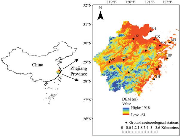
Figure 1 Positions of Zhejiang Province and the 12 stations used in this research.
3.2.3 CMFD
The background fields of China meteorological forcing dataset (CMFD) consist of Princeton reanalysis data, Global Land Data Assimilation System data, Tropical Rainfall Measuring Mission precipitation data, and Global Energy and Water Exchanges Project – Surface Radiation Budget (GEWEX-SRB) radiation data [27]. The CMFD dataset was created by integrating observation data from the China Meteorological Administration into these background fields. Among the components of the CMFD dataset are near-surface air temperature, near-surface air pressure, downward shortwave radiation, downward longwave radiation, specific humidity, wind speed, and precipitation rate. The dataset has a temporal resolution of 3 hours and daily intervals, along with a spatial resolution of 0.1∘ [28]. The time period of dataset is from 1979 to 2018. In this research, near-surface air temperature and precipitation rate are utilized.
3.2.4 GLEAM
The Global Land Evaporation Amsterdam Model (GLEAM) consists of a set of algorithms that are powered by satellite-based observations. These algorithms separately calculate the different elements of evapotranspiration (ET), such as snow sublimation, transpiration, bare soil evaporation, interception loss, and open-water evaporation [29, 30]. Otherwise, intermediate outputs of GLEAM include several variables, such as potential ET (PET), root-zone soil moisture, and surface soil moisture [31, 32]. Unlike previous GLEAM versions, GLEAM4 utilizes Penman’s equation to show the impact of various meteorological elements on potential evaporation. For this research, the monthly GLEAM_v4.2a dataset at a 0.1∘ resolution spanning from 1980 to 2018 is utilized. This dataset can be downloaded without charge from (https://www.gleam.eu) [30]. Three outputs (ET, PET, and surface soil moisture) are adopted in this study.
3.3 Methods
3.3.1 SPEI
Drought is not only affected by precipitation but also greatly influenced by evapotranspiration. SPEI was developed by Vicente-Serrano et al. [33] on the basis of the difference between precipitation and evapotranspiration. Furthermore, three-parameter log-logistic probability distribution functions are utilized in SPEI to reveal its changes. Subsequently, after normal normalization, the cumulative frequency distribution of the difference between standardized precipitation and evapotranspiration is ultimately utilized to categorize drought levels.
The common temporal resolutions of SPEI are 1, 3, 6,12, and 24 months. Three-month temporal resolution (SPEI3) is selected in this study and calculated in the following way:
(1) PET is computed using the Penman–Monteith equation.
The method recommended by Vicente-Serrano et al. [33] for computing PET is the Thornthwaite equation. Compared with the Penman–Monteith equation, this approach demands less data. As stated by Pan et al. [34], the Thornthwaite equation is less accurate than the Penman–Monteith equation. Thus, the Penman–Monteith equation is utilized to calculate the PET, and the details are provided by Allen et al. [35].
(2) The variance between monthly precipitation and PET is computed using the following equation:
| (1) |
where is the monthly precipitation, and represents the monthly PET. Here, i stands for the month. The climate water balance accumulation over a three-month period is established using the following equation:
| (2) |
where n stands for the number of calculations. Meanwhile, r is the temporal resolution, which is 3 for the three-month SPEI in this study.
(3) The values of Di are normalized, and the corresponding SPEI for each value is computed. Given that negative values may exist in Di sequence, log-logistic probability distribution functions of three parameters are used in SPEI and shown as follows:
| (3) |
Equation (3) contains three parameters, namely, , , and , which are acquired via fitting in accordance with the linear moment.
(4) The sequence to achieve the SPEI value is normalized as follows:
| (4) |
The probability of weight moments in Equation (4) is . When , ; when , .
First, observed daily meteorological data at 12 stations are used to calculate PET via the Penman–Monteith method, which yields the monthly PET. Based on the monthly PET and observed monthly precipitation, we calculate the observation-based SPEI3. Typically, the drought classification by SPEI is categorized into five levels, as listed in Table 2 [33].
Table 2 Criteria for grading drought in the SPEI3 classification
| Grade | Drought | SPEI |
| 1 | No drought | |
| 2 | Light drought | |
| 3 | Moderate drought | |
| 4 | Severe drought | |
| 5 | Extreme drought |
3.3.2 BP neural network
In this research, a commonly utilized machine learning algorithm – the BP neural network – is adopted to simulate the SPEI3. Renowned for its capability to approximate complex nonlinear functions, BP is a classic feedforward neural network model composed of multiple layers [36]. Its typical structure consists of three distinct layers: input, hidden, and output layers [37]. BP operates through forward propagation of input signals, followed by backward propagation of error gradients to adjust weights [38]. In this paper, three hidden layers were used in the BP neural network, with eight, fifteen, and nine neurons in the first, second, and third hidden layers, respectively.
3.3.3 Accuracy assessment
Multiple statistical metrics, such as the Nash–Sutcliffe efficiency (NSE), root mean square error (RMSE), and correlation coefficient (R), are employed to comprehensively evaluate the performance of the BP model in SPEI3 estimation. These metrics can be computed using the following equations.
| (5) | ||
| (6) | ||
| (7) |
where n is the sample size of data, Oi and Si are the ith values of observed SPEI3 and predicted SPEI3 via the BP model, respectively. represents the mean of the observed SPEI3 values, whereas denotes the mean of the SPEI3 values predicted by the BP model. The optimal values of NSE, RMSE, and R are 1.0, 0, and 1.0, respectively.
4 Results Analysis and Discussion
4.1 Combination of Inputs and Implementation of the Model
In theory, drought is usually affected by vegetation greenness, climate conditions, and soil moisture. Thus, this study adopted eight related variables, namely, precipitation (P), surface temperature (T), actual evapotranspiration (ET), leaf area index (LAI), PET, soil moisture (SM), difference between precipitation and actual ET (P-ET), and difference between precipitation and PET (P-PET). Subsequently, four variables (P, SM, P-ET, and P-PET) were initially selected based on their correlation coefficients (R 0.5) with SPEI3, as presented in Table 3. Considering the similar meaning of P-ET and P-PET, P-PET is finally selected due to its little higher correlation coefficient than P-ET. Therefore, three variables (P, SM, and P-PET) are ultimately employed as input variables. Table 4 displays the seven input combinations utilized in the BP model. The target of all combinations is a single response, that is, SPEI3. Three schemes are established from these input combinations. They are single-variable input (Scheme I), two-variable input (Scheme II), and three-variable input (Scheme III). The exploration of the optimal input combinations for each of these schemes is the objective in this research. By contrasting these combinations, the optimal one for each station would be subsequently acquired.
Table 3 Correlation coefficient (R) between input variables and SPEI3
| Stations | ||||||||||||
| Variables | HZ | PH | CX | DH | JH | SX | YX | SP | QZ | LS | HJ | YH |
| P | 0.68 | 0.65 | 0.67 | 0.60 | 0.75 | 0.72 | 0.73 | 0.68 | 0.78 | 0.79 | 0.78 | 0.75 |
| T | 0.18 | 0.18 | 0.20 | 0.13 | 0.34 | 0.20 | 0.02 | 0.07 | 0.30 | 0.13 | 0.22 | 0.00 |
| LAI | 0.07 | 0.02 | 0.04 | 0.05 | 0.09 | 0.06 | 0.03 | 0.10 | 0.15 | 0.16 | 0.03 | 0.10 |
| ET | 0.16 | 0.14 | 0.19 | 0.12 | 0.23 | 0.14 | 0.01 | 0.08 | 0.14 | 0.01 | 0.28 | 0.21 |
| PET | 0.18 | 0.19 | 0.23 | 0.12 | 0.30 | 0.17 | 0.01 | 0.03 | 0.27 | 0.14 | 0.24 | 0.10 |
| SM | 0.60 | 0.55 | 0.49 | 0.46 | 0.64 | 0.62 | 0.60 | 0.67 | 0.58 | 0.65 | 0.63 | 0.62 |
| P-ET | 0.90 | 0.89 | 0.92 | 0.85 | 0.94 | 0.92 | 0.90 | 0.87 | 0.90 | 0.93 | 0.87 | 0.87 |
| P-PET | 0.91 | 0.91 | 0.94 | 0.85 | 0.95 | 0.94 | 0.90 | 0.89 | 0.90 | 0.94 | 0.88 | 0.88 |
Table 4 Combinations of inputs according to selected variables
| Input Combination | Input Variables | Abbreviations |
| Scheme I | P | P |
| SM | S | |
| P-PET | PE | |
| Scheme II | P, SM | PS |
| P, P-PET | PPE | |
| SM, P-PET | SPE | |
| Scheme III | P, SM, P-PET | PSPE |
4.2 Impacts of Various Input Combinations on SPEI Estimation
4.2.1 Single-variable input
In this section, the initial input combination scheme (Scheme I) is employed independently. This plan involves single-variable input (comprising P, S, and PE). Specifically, three input combinations are used in this section. To explore the uncertainty of the BP model, for each input combination, the model is run repeatedly 100 times. For each run, the NSE is computed using the BP-predicted SPEI3 and the observed SPEI3 during the test period, and its distribution is displayed Figure 2. As depicted in Figure 2, notable variations in model performance are observed across the different input combinations within Scheme I. PE has the optimal performance in Scheme I, P is the second, and S performs the worst.
For the optimal input combination at each station in Scheme I, their performances are listed in Table 5. Besides the DH station, 11 other stations show great performances, which are characterized by high NSE values exceeding 0.80, R values greater than 0.90, and low RMSE values below 0.45. The slightly poor performance at the DH station is mainly due to that the correlation coefficient between PE and SPEI3 is slightly lower.
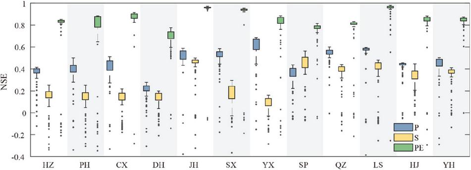
Figure 2 Performance of the BP model based on Scheme I at 12 stations.
Table 5 Best input combinations in Scheme I and their performances at 12 stations
| Stations | Combination | NSE | RMSE | R |
| HZ | PE | 0.85 | 0.37 | 0.94 |
| PH | PE | 0.88 | 0.34 | 0.94 |
| CX | PE | 0.91 | 0.33 | 0.96 |
| DH | PE | 0.78 | 0.58 | 0.92 |
| JH | PE | 0.97 | 0.17 | 0.99 |
| SX | PE | 0.95 | 0.23 | 0.98 |
| YX | PE | 0.88 | 0.37 | 0.94 |
| SP | PE | 0.81 | 0.44 | 0.90 |
| QZ | PE | 0.83 | 0.43 | 0.91 |
| LS | PE | 0.98 | 0.13 | 0.99 |
| HJ | PE | 0.88 | 0.33 | 0.94 |
| YH | PE | 0.87 | 0.33 | 0.94 |
4.2.2 Two-variable input
For the simulation of SPEI3 using the BP model in this part, the second scheme of input combinations (referred to as Scheme II), which involves two input variables, is adopted. Three input combinations, as shown in Table 3, are applied in this section. Similar to Scheme I, for each input combination, the model is executed repeatedly 100 times to explore its uncertainty. For each run, the NSE is computed using the BP-predicted SPEI3 and the observed SPEI3 during the test period, and its distribution is displayed Figure 3. As shown in Figure 3, the differences in Scheme II are much lower than those in Scheme I. In Scheme II, PPE and SPE have comparable performances and outperform PS.
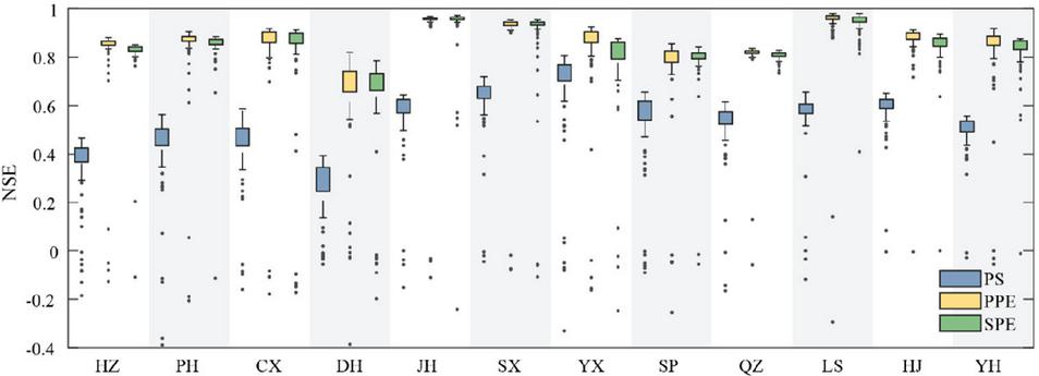
Figure 3 Performance of the BP model based on Scheme II at 12 stations.
Table 6 Optimal input combinations within Scheme II and their performances at 12 stations
| Stations | Combination | NSE | RMSE | R |
| HZ | PPE | 0.88 | 0.33 | 0.95 |
| PH | PPE | 0.90 | 0.31 | 0.95 |
| CX | PPE | 0.92 | 0.33 | 0.97 |
| DH | PPE | 0.82 | 0.52 | 0.92 |
| JH | SPE | 0.97 | 0.17 | 0.99 |
| SX | PPE | 0.95 | 0.23 | 0.98 |
| YX | PPE | 0.93 | 0.29 | 0.96 |
| SP | PPE | 0.85 | 0.38 | 0.93 |
| QZ | PPE | 0.84 | 0.43 | 0.92 |
| LS | PPE | 0.98 | 0.13 | 0.99 |
| HJ | PPE | 0.91 | 0.29 | 0.96 |
| YH | PPE | 0.92 | 0.27 | 0.96 |
When the performances of three input combinations are compared, the optimal input combinations in Scheme II for 12 stations are acquired (Table 6). Except for the JH station, the optimal input combinations in Scheme II at the other stations are PPE. Actually, at the JH station, the NSE values for PPE and SPE are 0.969 and 0.973, respectively. As presented in Tables 5 and 6, the optimal input combinations in Scheme II demonstrate superior performance relative to those in Scheme I. In Scheme II, the NSE values at the 12 stations vary from 0.82 to 0.98, the RMSE values span from 0.13 to 0.52, and the R values vary between 0.92 and 0.99. Especially at the DH station, the NSE value in Scheme II is 0.82 (the NSE value in Scheme I is 0.78), the RMSE value in Scheme II is 0.52 (the RMSE value in Scheme I is 0.58), and the R value in Scheme II is 0.92 (the R value in Scheme I is 0.92).
4.2.3 Three-variable input
In this section, all three input variables (Scheme III) are employed. Similar to Schemes I and II, the BP model is executed repeatedly 100 times to explore its uncertainty. In contrast to Figures 2 to 4, the performance difference decreases as the number of input variables increases.
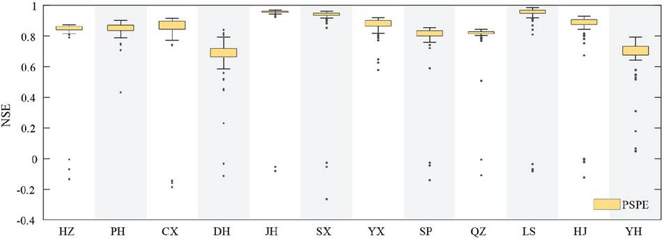
Figure 4 Performance of the BP model based on Scheme III at 12 stations.
Table 7 Performance of Scheme III at 12 stations
| Stations | Combination | NSE | RMSE | R |
| HZ | PSPE | 0.87 | 0.34 | 0.95 |
| PH | PSPE | 0.90 | 0.32 | 0.95 |
| CX | PSPE | 0.92 | 0.33 | 0.97 |
| DH | PSPE | 0.84 | 0.49 | 0.93 |
| JH | PSPE | 0.97 | 0.17 | 0.99 |
| SX | PSPE | 0.96 | 0.20 | 0.98 |
| YX | PSPE | 0.92 | 0.30 | 0.96 |
| SP | PSPE | 0.85 | 0.39 | 0.93 |
| QZ | PSPE | 0.84 | 0.42 | 0.92 |
| LS | PSPE | 0.99 | 0.12 | 0.99 |
| HJ | PSPE | 0.93 | 0.26 | 0.96 |
| YH | PSPE | 0.92 | 0.26 | 0.96 |
Table 7 presents the performance results of Scheme III across 12 stations. Six stations (DH, SX, QZ, LS, HJ, and YH) perform better in Scheme III than those in Scheme II, while the six other stations are the opposite. Among the schemes evaluated, the improvement observed at the DH station is most pronounced in Scheme III than in Scheme II. At the DH station, the NSE value of Scheme III is 0.84 (NSE of Scheme II: 0.82), the RMSE value of Scheme III is 0.49 (RMSE of Scheme II: 0.52), and the R value of Scheme III is 0.93 (R of Scheme II: 0.92). Based on the data from the HZ, PH, CX, JH, YX, and SP stations, adding more input variables does not always guarantee better performance.
Table 8 Optimal input combinations in Schemes I to III at 12 stations
| Scheme I | Scheme II | Scheme III | ||||
| Stations | Combination | NSE | Combination | NSE | Combination | NSE |
| HZ | PE | 0.85 | PPE | 0.88 | PSPE | 0.87 |
| PH | PE | 0.88 | PPE | 0.90 | PSPE | 0.90 |
| CX | PE | 0.91 | PPE | 0.92 | PSPE | 0.92 |
| DH | PE | 0.78 | PPE | 0.82 | PSPE | 0.84 |
| JH | PE | 0.97 | SPE | 0.97 | PSPE | 0.97 |
| SX | PE | 0.95 | PPE | 0.95 | PSPE | 0.96 |
| YX | PE | 0.88 | PPE | 0.93 | PSPE | 0.92 |
| SP | PE | 0.81 | PPE | 0.85 | PSPE | 0.85 |
| QZ | PE | 0.83 | PPE | 0.84 | PSPE | 0.84 |
| LS | PE | 0.98 | PPE | 0.98 | PSPE | 0.99 |
| HJ | PE | 0.88 | PPE | 0.91 | PSPE | 0.93 |
| YH | PE | 0.87 | PPE | 0.92 | PSPE | 0.92 |
| Note: The highlighted term in each data entry denotes the optimal input combination for the respective station. | ||||||
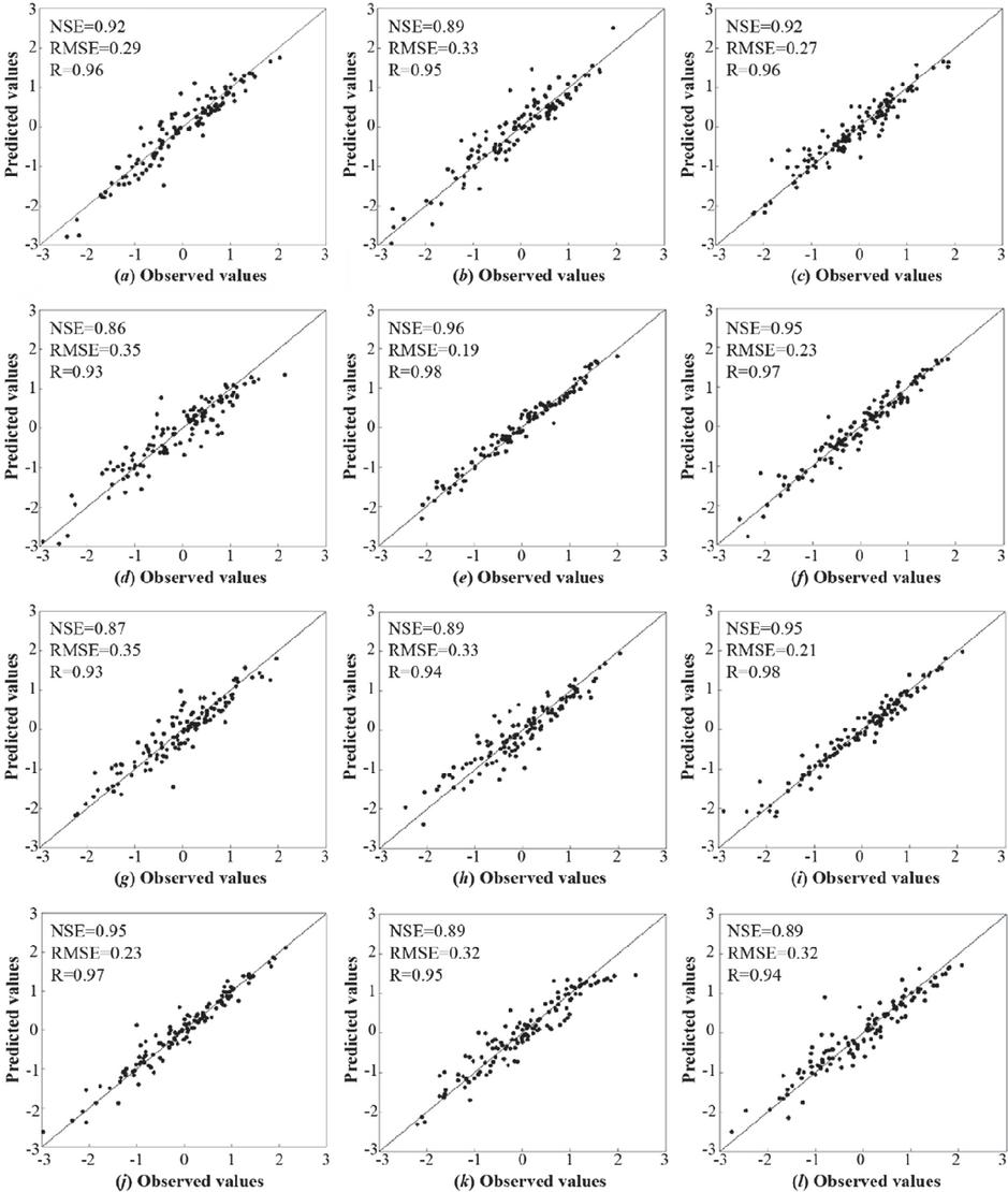
Figure 5 Scatterplot of the BP model predictions with observations in the training period. (a–l) correspond to the 12 stations.
4.3 BP Model Performances for SPEI Estimation based on the Optimal Input Combinations
Tables 5 to 7 have been synthesized to identify the optimal input combinations for the 12 stations, which are emphasized in bold in Table 8. They correspond to the maximum NSE value achieved during the testing phase. Figures 5 and 6 present scatter plots comparing observed SPEI3 values with those predicted by the BP model for the training and testing periods across the 12 stations, utilizing their respective optimal input combinations. As demonstrated in the two figures, the predicted SPEI3 values exhibit a satisfactory degree of agreement with the observed data throughout both phases. Furthermore, Figure 7, which illustrates the temporal sequence of observed and predicted SPEI3 data at the 12 stations, supports a similar conclusion. Regarding the temporal variation aspect, the predicted SPEI3 demonstrates excellent capabilities in reflecting the trends of the observed SPEI3 at 12 stations during the training and testing phases.
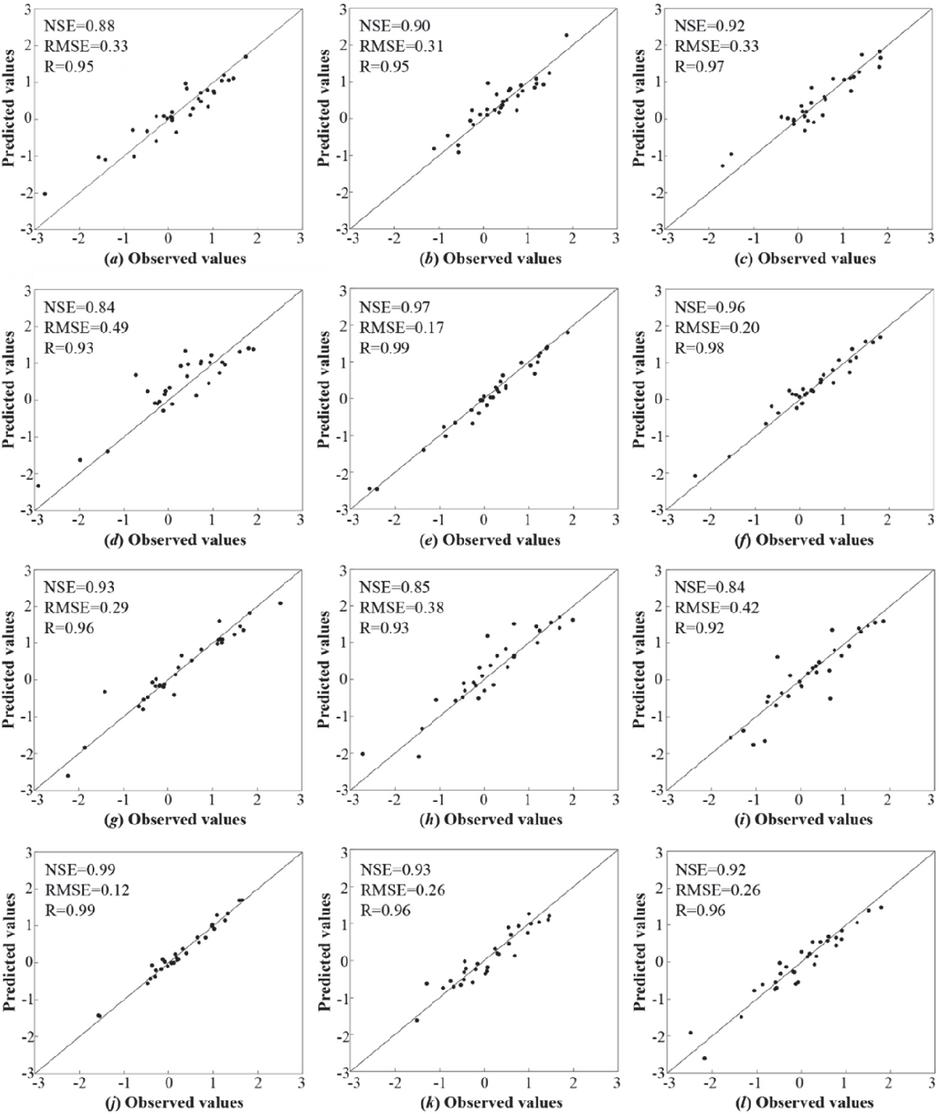
Figure 6 Scatterplot of the BP model predictions with observations in the test period. (a–l) correspond to the 12 stations.
Across all 12 stations, the BP model demonstrates the greatest precision at the LS, JH, and SX stations, with the NS value exceeding 0.95. This station is followed by the PH, CX, YX, HJ, and YH stations, where the NS values range between 0.90 and 0.95. Finally, the HZ, DH, SP, and QZ stations exhibit NS values between 0.84 and 0.90. These values indicate comparatively lower model performance at these locations. The 12 stations are evenly distributed in Zhejiang Province. Combining the spatial distribution of 12 stations and the performances of the BP model shows that the performances of the BP model in inland stations are slightly better than those in costal stations. The primary reason for this phenomenon lies in complex and multifaceted influencing factors in costal stations, such as wave action, atmospheric river, and monsoon system. These results show that the performance of the model varies across different stations.
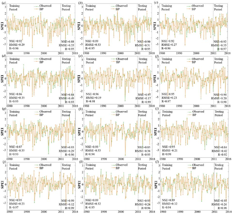
Figure 7 Comparation between SPEI3 computed from observed data and that predicted by the BP model in the training period and testing period. (a–l) correspond to the 12 stations.
4.4 Discussion
In this study, the BP model uses three input variables – precipitation, soil moisture, and difference between precipitation and PET – to simulate SPEI3. According to these variables, the input combinations are divided into three schemes: single-variable input (Scheme I), two-variable input (Scheme II), and three-variable input (Scheme III). Initially, the optimal input combinations for each of the mentioned schemes are investigated. Subsequently, by making a comparison among these combinations, the optimal input combinations for the various stations are determined.
As presented in Table 5, in Scheme I, the optimal input combination across all stations is PE. This selection is primarily attributed to that the correlation coefficient between PE and SPEI3 reaches the maximum value. The relatively poor performance observed at the DH station can primarily be attributed to the low correlation coefficient between PE and SPEI3. At the DH stations, the correlation coefficient between PE and SPEI3 is 0.85. Meanwhile, at the other stations, the correlation coefficients are mostly greater than 0.90. In general, single-variable input can predict SPEI3 very well via the BP model at most stations. For Scheme II, PPE and SPE have comparably performances for simulating SPEI3 at most stations (Figure 3), which is mainly due to PPE and SPE containing PE. Compared with the best combination in Scheme I, the performance of the optimal combination in Scheme II has relatively improved, with increases in NSE and R and a decrease in RMSE. Therefore, adding sensitive input variables contributes to the improvement in the BP performance in general.
For Scheme III (Table 8), an increase in input variables does not necessarily result in improved performance, as evidenced by the HZ, PH, CX, JH, YX, and SP stations. This finding supports the conclusion drawn by Mokhtar et al. [22], but it contradicts the outcome of Tao et al. [39]. Mokhtar et al. [22] adopted four machine learning methods to estimate SPEI3 based on seven scenarios. The results demonstrated that the corresponding input scenarios for the best performances for SPEI3 were not the scenarios with all input variables. A new hybrid ANFIS-FA model in Tao et al. [39] was applied to evaluate reference evapotranspiration based on diverse meteorological elements. The findings indicated that the optimal accuracy was attained with a combination of six input variables. Nevertheless, only six input combinations were used in Tao et al. [39], that is, one meteorological element was added to the preceding combination to obtain the subsequent combination. All possible combinations cannot be obtained in this way, and some may represent the best combination. Thus, an increased quantity of input variables does not result in enhanced performance. Moreover, Zhao et al. [17] utilized three machine learning models to forecast SPEI3 only based on one combination, that is, six input variables (i.e., precipitation, soil moisture, temperature, ET, PET, and vegetation index). The results exhibited that this input combination could accurately predict SPEI3. That is, Zhao et al. [17] did not test other input variable combinations, which may obtain better performance. Thus, multiple input variable combinations should be compared to obtain the best combination.
5 Conclusions
Under three combinations of input variables (single-variable input, two-variable input, and three-variable input), the BP model is utilized to predict SPEI3 in Zhejiang Province in this research. The main conclusions of this research are presented as follows:
(1) The BP model, which is a machine learning model, is proven to be an effective approach for predicting SPEI3 in Zhejiang Province, China. It shows high NSE values ranging from 0.84 to 0.99, high R values from 0.92 to 0.99, and low RMSE values from 0.12 to 0.42.
(2) In general, a greater number of input variables can result in enhanced performance of the BP model when predicting SPEI3. The performances improve obviously from Schemes I to II, and the performances of the BP model are slightly enhanced at half of the stations between Schemes II and III.
(3) The analysis of BP performance across six stations reveals that an increase in the number of input variables does not inherently result in enhanced outcomes. At these stations, the BP model under two-variable input outperforms those under three-variable input.
(4) The differential performance of the BP model across 12 stations suggests that various factors, including altitude and types of vegetation cover, affect the accuracy of SPEI3 predictions. Furthermore, the inclusion of additional input variables, such as wind speed, air temperature, and LAI, has the potential to enhance the predictive capability of the SPEI3 model.
Acknowledgements
The authors are grateful for the support provided by the Water Conservancy Science and Technology Project of Hunan Province (Grant No. XSKJ2024064-49), the Science Project of Zhejiang Institute of Hydraulics & Estuary (Grant No. FZJZSYS21006), the Key Project Fund of Zhejiang Institute of Hydraulics and Estuary (Grant No. ZIHE21Z007), and the Zhejiang Provincial Basic Public Welfare Research Program (Grant No. LTGS23E090004).
References
[1] S. Lee, D. N. Moriasi, A. Danandeh Mehr, and A. Mirchi, “Sensitivity of standardized precipitation and evapotranspiration index (SPEI) to the choice of SPEI probability distribution and evapotranspiration method,” J. Hydrol. Reg. Stud., vol. 53, p. 101761, June 2024.
[2] A. Abu Arra and E. Şişman, “A comprehensive analysis and comparison of SPI and SPEI for spatiotemporal drought evaluation,” Environ. Monit. Assess., vol. 196, no. 10, p. 980, Oct. 2024.
[3] V. Gumus, “Evaluating the effect of the SPI and SPEI methods on drought monitoring over turkey,” J. Hydrol., vol. 626, p. 130386, Nov. 2023.
[4] J. Uwimbabazi, Y. Jing, V. Iyakaremye, I. Ullah, and B. Ayugi, “Observed changes in meteorological drought events during 1981–2020 over rwanda, east africa,” Sustainability, vol. 14, no. 3, p. 1519, Jan. 2022.
[5] W. Zhang et al., “Temporal and spatial evolution of meteorological drought in inner mongolia inland river basin and its driving factors,” Sustainability, vol. 16, no. 5, p. 2212, Mar. 2024.
[6] B. Ayugi et al., “Review of meteorological drought in africa: Historical trends, impacts, mitigation measures, and prospects,” Pure Appl. Geophys., vol. 179, no. 4, pp. 1365–1386, Apr. 2022.
[7] A. A. Pathak and B. M. Dodamani, “Connection between meteorological and groundwater drought with copula-based bivariate frequency analysis,” J. Hydrol. Eng., vol. 26, no. 7, p. 05021015, July 2021.
[8] R. Xue et al., “Future projections of meteorological, agricultural and hydrological droughts in China using the emergent constraint,” J. Hydrol. Reg. Stud., vol. 53, p. 101767, June 2024.
[9] T. Lan and X. Yan, “Analysis of drought characteristics and causes in yunnan province in the last 60 years (1961–2020),” J. Hydrometeorol., vol. 25, no. 1, pp. 177–190, Jan. 2024.
[10] L. Zhang et al., “Dynamic multi-dimensional identification of yunnan droughts and its seasonal scale linkages to the el niño-southern oscillation,” J. Hydrol. Reg. Stud., vol. 42, p. 101128, Aug. 2022.
[11] Z. Hao, D. Xiong, and J. Zheng, “How ancient China dealt with summer droughts – a case study of the whole process of the 1751 drought in the qing dynasty,” Clim. Change, vol. 165, no. 1–2, p. 16, Mar. 2021.
[12] I. J. Nwayor and S. M. Robeson, “Exploring the relationship between SPI and SPEI in a warming world,” Theor. Appl. Climatol., vol. 155, no. 4, pp. 2559–2569, Apr. 2024.
[13] A. Merabti, H. Darouich, P. Paredes, M. Meddi, and L. S. Pereira, “Assessing spatial variability and trends of droughts in eastern algeria using SPI, RDI, PDSI, and MedPDSI – a novel drought index using the FAO56 evapotranspiration method,” Water, vol. 15, no. 4, p. 626, Feb. 2023.
[14] M. Kamruzzaman et al., “Spatiotemporal drought analysis in bangladesh using the standardized precipitation index (SPI) and standardized precipitation evapotranspiration index (SPEI),” Sci. Rep., vol. 12, no. 1, p. 20694, Nov. 2022.
[15] D. C. D. Melo et al., “Are remote sensing evapotranspiration models reliable across south American ecoregions?,” Water Resour. Res., vol. 57, no. 11, p. e2020WR028752, Nov. 2021.
[16] S. Wanniarachchi and R. Sarukkalige, “A review on evapotranspiration estimation in agricultural water management: Past, present, and future,” Hydrology, vol. 9, no. 7, p. 123, July 2022.
[17] Y. Zhao et al., “Drought monitoring and performance evaluation based on machine learning fusion of multi-source remote sensing drought factors,” Remote Sens., vol. 14, no. 24, p. 6398, Dec. 2022.
[18] H. Zhao, Y. Huang, X. Wang, X. Li, and T. Lei, “The performance of SPEI integrated remote sensing data for monitoring agricultural drought in the north China plain,” Field Crops Res., vol. 302, p. 109041, Oct. 2023.
[19] P. S. Wable, M. K. Jha, S. Adamala, M. K. Tiwari, and S. Biswal, “Application of hybrid ANN techniques for drought forecasting in the semi-arid region of India,” Environ. Monit. Assess., vol. 195, no. 9, p. 1090, Sept. 2023.
[20] M. S. Oyounalsoud, A. G. Yilmaz, M. Abdallah, and A. Abdeljaber, “Drought prediction using artificial intelligence models based on climate data and soil moisture,” Sci. Rep., vol. 14, no. 1, p. 19700, Aug. 2024.
[21] T. Yildirim, D. N. Moriasi, P. J. Starks, and D. Chakraborty, “Using artificial neural network (ANN) for short-range prediction of cotton yield in data-scarce regions,” Agronomy, vol. 12, no. 4, p. 828, Mar. 2022.
[22] A. Mokhtar et al., “Estimation of SPEI meteorological drought using machine learning algorithms,” IEEE Access, vol. 9, pp. 65503–65523, 2021.
[23] B. Poudel, D. Dahal, M. Banjara, and A. Kalra, “Assessing meteorological drought patterns and forecasting accuracy with SPI and SPEI using machine learning models,” Forecasting, vol. 6, no. 4, pp. 1026–1044, Nov. 2024.
[24] Y. Xu, S. Pan, G. Fu, Y. Tian, and X. Zhang, “Future potential evapotranspiration changes and contribution analysis in zhejiang province, east China,” J. Geophys. Res. Atmospheres, vol. 119, no. 5, pp. 2174–2192, Mar. 2014.
[25] M. Ghaderi and M. Rahimzadegan, “Improving precipitable water vapor estimations of the moderate resolution imaging spectroradiometer (MODIS) using metaheuristic algorithms,” Adv. Space Res., vol. 69, no. 12, pp. 4274–4287, June 2022.
[26] S. Kloos, Y. Yuan, M. Castelli, and A. Menzel, “Agricultural drought detection with MODIS based vegetation health indices in southeast germany,” Remote Sens., vol. 13, no. 19, p. 3907, Jan. 2021.
[27] K. Yang et al., “China meteorological forcing dataset v1.6 (1979–2018).” National Tibetan Plateau Data Center, 2019.
[28] K. Yang, J. He, W. Tang, J. Qin, and C. C. K. Cheng, “On downward shortwave and longwave radiations over high altitude regions: Observation and modeling in the tibetan plateau,” Agric. For. Meteorol., vol. 150, no. 1, pp. 38–46, Jan. 2010.
[29] D. G. Miralles, R. A. M. De Jeu, J. H. Gash, T. R. H. Holmes, and A. J. Dolman, “Magnitude and variability of land evaporation and its components at the global scale,” Hydrol. Earth Syst. Sci., vol. 15, no. 3, pp. 967–981, Mar. 2011.
[30] D. G. Miralles et al., “GLEAM4: Global land evaporation and soil moisture dataset at 0.1∘ resolution from 1980 to near present,” Sci. Data, vol. 12, no. 1, p. 416, Mar. 2025.
[31] J. Liu, J. Zhang, D. Kong, X. Feng, S. Feng, and M. Xiao, “Contributions of anthropogenic forcings to evapotranspiration changes over 1980–2020 using GLEAM and CMIP6 simulations,” J. Geophys. Res. Atmospheres, vol. 126, no. 22, p. e2021JD035367, Nov. 2021.
[32] X. Yang, B. Yong, L. Ren, Y. Zhang, and D. Long, “Multi-scale validation of GLEAM evapotranspiration products over China via ChinaFLUX ET measurements,” Int. J. Remote Sens., vol. 38, no. 20, pp. 5688–5709, Oct. 2017.
[33] S. M. Vicente-Serrano, S. Beguería, and J. I. López-Moreno, “A multiscalar drought index sensitive to global warming: The standardized precipitation evapotranspiration index,” J. Clim., vol. 23, no. 7, pp. 1696–1718, Apr. 2010.
[34] S. Pan, Y.-P. Xu, W. Xuan, H. Gu, and Z. Bai, “Appropriateness of potential evapotranspiration models for climate change impact analysis in yarlung zangbo river basin, China,” Atmosphere, vol. 10, no. 8, p. 453, Aug. 2019.
[35] R. G. Allen, M. Smith, A. Perrier, and L. S. Pereira, “An update for the calculation of potential evapotranspiration,” ICID Bull, vol. 43, pp. 35–92, 1994.
[36] L. Zhao et al., “Prediction model for reference crop evapotranspiration based on the back-propagation algorithm with limited factors,” Water Resour. Manag., vol. 37, no. 3, pp. 1207–1222, Feb. 2023.
[37] Z. Zhang, Y. Gong, and Z. Wang, “Accessible remote sensing data based reference evapotranspiration estimation modelling,” Agric. Water Manag., vol. 210, pp. 59–69, Nov. 2018.
[38] Y. Gong, Y. Zhang, S. Lan, and H. Wang, “A comparative study of artificial neural networks, support vector machines and adaptive neuro fuzzy inference system for forecasting groundwater levels near lake okeechobee, florida,” Water Resour. Manag., vol. 30, no. 1, pp. 375–391, Jan. 2016.
[39] H. Tao, L. Diop, A. Bodian, K. Djaman, P. M. Ndiaye, and Z. M. Yaseen, “Reference evapotranspiration prediction using hybridized fuzzy model with firefly algorithm: Regional case study in burkina faso,” Agric. Water Manag., vol. 208, pp. 140–151, Sept. 2018.
Biographies

Zuisen Li received his Ph.D. degree in Regional and Built Environment Science from Kobe University, Japan, in 2007. He is currently a professor of engineering at Zhejiang Institute of Hydraulics and Estury in China. His research areas include engineering hydrology, river dynamics, and marine surveying.

Yan Liu is an associate professor at Hunan Polytechnic of Water Resources and Electric Power in Hunan Province, China. She has long been dedicated to teaching and research in hydraulic engineering, with a focus on safety assessment and the intelligent construction of hydraulic projects. She has published several research papers in related academic journals.

Zhao Sun obtained a master’s degree in hydraulic engineering from Hohai University, China, in 2016. He is currently a senior engineer at Ningbo Datong Development Co., Ltd., primarily engaged in research and application of construction management technologies in water transportation engineering.

Lihui Chen is currently a senior engineer at the Zhejiang Provincial Hydrology Management Center in China. He is primarily responsible for the construction and management of digital infrastructure for hydrological monitoring and has extensive experience in research on hydrological data analysis and mining.
Strategic Planning for Energy and the Environment, Vol. 45_1, 179–204
doi: 10.13052/spee1048-5236.4517
© 2026 River Publishers