Enhanced Analysis of PV Array Operating in Partial Shading Conditions Using a Dispersed Illumination Technique

AL Shifa Kafeel, Zeeshan Ali Khan and Mohd Faisal Jalil^*

Department of Electrical Engineering, Zakir Husain College of Engineering and Technology, Aligarh Muslim University, Aligarh, India
E-mail: mohdfaisaljalil@zhcet.ac.in
*Corresponding Author

Received 25 November 2025; Accepted 24 April 2026

Abstract

Partial shading of a PV array leads to lower energy yield and results in multiple peaks in its P–V characteristics. The losses due to partial shading are not proportional to the shaded area but are dependent on the shading pattern, array configuration and the physical position of shaded modules in the array. This paper presents a novel Dispersed Illumination (DI) technique for mitigating partial shading effects in a Total Cross-Tied (TCT) photovoltaic (PV) array configuration. The proposed technique aims to maximize power output under various partial shading conditions by physically redistributing shaded modules across the array, thereby reducing the mismatch losses and suppressing the formation of multiple local maxima in the power–voltage characteristics. The simulation results have been compared to the Odd–Even and TCT configuration results. The proposed technique consistently outperforms both the Odd–Even and conventional TCT arrangements by delivering higher maximum power output, thereby demonstrating its superior effectiveness in mitigating partial shading losses. Owing to its simplicity, the proposed method offers a practical and efficient solution for improving PV array performance in real-world partially shaded environments.

Keywords: Dispersed illumination, partial shading, photovoltaic, local maxima, total cross tied.

1 Introduction

Global warming and air pollution are two of the biggest issues facing environmentalists worldwide. The reliance on fossil fuels is a significant factor contributing to this issue. Meanwhile, the ecosystem is being severely harmed and fossil fuel reserves are being depleted more and more every day. Sustainable development can be achieved through the limitless supply and generation of electricity from solar photovoltaic panels. Solar PV technology has become extremely powerful and rapidly expanding on a worldwide basis in recent years, from modest rooftop power plants to several MW power plants [1]. However, a practical PV system has to capture as much energy as possible due to the low conversion efficiency of the PV cell [2]. As a result, renewable energy sources, particularly photovoltaic (PV) or solar energy, are becoming increasingly popular [3]. Crystalline, thin-film, compound, and nanotechnology are the four widely used PV technologies [4]. The effectiveness of solar photovoltaic (PV) cells is diminished by various losses. When sunlight is transmitted, meditated, or obscured by shade, optical losses take place. When excess photon energy is converted to heat rather than electricity, thermal losses take place, and additional heating is brought on by resistance inside the circuit. Variations among sun cells, high temperatures that impair performance, and strength losses in wiring and inverters are examples of mismatch and device losses. These mismatch-related losses need to be addressed to increase the energy yield of photovoltaic (PV) systems [5, 6]. Over the past few decades, the cost of generating power per unit has decreased exponentially because to advancements in PV technology [7]. Partial shading losses are one of the main contributors to the PV device’s losses. Partial shading causes mismatch losses, which ultimately lowers the PV module’s total power yield [8]. Moving modules in and out of the shade is known as array reconfiguration, and it is a crucial approach to reduce these losses [9, 10]. Due to passing clouds, adjacent PV modules, birds, etc., large PV plants spread out over a large region may face partial shade or an imbalance in the array’s irradiance [11]. Moreover, aging and cracking of PV cells can cause shading [12]. As a result, the photovoltaic cell starts to act as a load, using a lot of electricity and then releasing it as heat. This process leads to the formation of hotspots [13].

Partial shading losses depend on the array structure, shading pattern, and the placement of shaded modules. One common mitigation approach is the installation of bypass diodes between solar cells or modules, which is one of the simplest and most widely used techniques. By enabling the current to avoid the shaded area of the module, bypass diodes lessen the effect of shading on the array’s overall performance.

PV cells or modules may sustain damage, and the PV system as a whole may be impacted by the mismatch loss that happens when shaded PV modules restrict an array’s output current [15]. Photovoltaic modules can be linked both in series and in parallel to form a photovoltaic array [16]. In order to achieve the required voltage, these modules are linked in series, while to obtain the needed current, they are arranged in parallel. A PV array consists of either a single module or multiple modules, arranged in both series and parallel configurations [17]. Various combinations enhance partial shading methods, including series-parallel (SP), bridge linked (BL), and total cross tied (TCT) [18, 19]. Extensive studies have demonstrated that when moving from SP to TCT, power generation increases by at least 5% when the module communication system is upgraded [20]. The authors in [21] also demonstrate the magic square, odd-even, and Auduko methods for partial shading. In [22], the author provides an example of a similar shade dispersal approach known as the Suduko method. Based on their GMPP, fill factor (FF), losses, dependability, and the power output drop brought on by partial shade, as well as the tolerance offered by different manufacturers, the aforementioned systems vary. As demonstrated by the author in [23], TCT is the best configuration among all of these for the partial shading scenario.

By carefully positioning modules in a PV array, this research presents a sophisticated Dispersed Illumination Technique for enhancing generation in partially shaded environments. By carefully redistributing the shading’s effects throughout the array, the suggested method reduces mismatch losses and boosts overall effectiveness. The DI technique prevents concentrated hotspots and lessens power degradation by ensuring a good dispersion of shaded and unshaded modules, in contrast to conventional arrangements. This method offers versatility in array architecture to optimize power harvesting, supporting both symmetrical and asymmetrical configurations. A thorough assessment of the DI method is conducted under a variety of shading scenarios, including tree shadows, shifting clouds, and adjacent obstacles.

The results indicate a notable enhancement in power output in comparison to traditional photovoltaic (PV) array systems, illustrating the efficiency of the suggested approach in minimizing losses associated with shading.

2 Photovoltaic Module

A single PV module is composed of multiple photovoltaic cells linked in series. The circuit model incorporates an anti-parallel diode, series resistance (R₁), parallel resistance (R₂), and a current source ($I_{\mathit{ph}}$). Figure 1 illustrates the equivalent circuit of the PV module.

$$I_m=I_{\mathit{ph}}-I_o\left[e^{q\left(\frac{V_{PV}+I_m{R}_1}{AkT}\right)}-1\right]-\left(\frac{V_{PV}+I_m{R}_1}{R_2}\right)$$

(1)

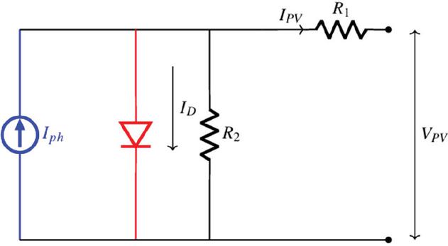
Figure 1 Equivalent circuit of the PV module.

The Equation (1) describes the current of a module [24] and is referred to as the five-parameter model. In this model, $I_{\mathit{ph}}$ signifies the current generated by photons, q represents the electron charge, which is 1.6 $\times$ 10–19 C, Io denotes the saturation current, $V_{\mathit{pv}}$ indicates the voltage of the panel, $I_m$ refers to the output current of the panel, A is the curve-fitting constant, K stands for the Boltzmann constant, T represents the temperature of the cell in Celsius, Rp is the shunt resistor, and Rs is the series resistor.

$$Iph=Iph,n(1+K_1\mathrm{\Delta }T)\frac{G}{Gn}$$

(2)

The photon generated current as presented [23] is given by Equation (2).

Where $Iph$ is the photocurrent produced at the actual irradiance and temperature, while $I_{\mathit{ph},n}$ denotes the photocurrent under standard test conditions. The factor $K_I$ is the temperature coefficient that shows how photocurrent changes with temperature and $\mathrm{\Delta }T$ is the difference between the cell temperature and its nominal value. The ratio $G/G_n$ accounts for the change in solar irradiance by scaling the photocurrent based on the available sunlight. Together, these terms show how changes in temperature and irradiance affect the output of the PV cell.

$$I_o=\frac{I_{sc},n+K1\mathrm{\Delta }T}{exp\left(\frac{v_{oc},n+Kv\mathrm{\Delta }T}{AVt}\right)-1}$$

(3)

The reverse saturation current follows complex relation given by Equation (3)

$$V_{\mathit{OC}}=V_{\mathit{OC}},n+Kv\mathrm{\Delta }T$$

(4)

The open circuit voltage is given by Equation (4).

3 Dispersed Illumination Technique

A method called the Dispersed Illumination technique of modules is presented in this study. The modules in this technique are connected in the same manner as in the TCT arrangement. The modules’ actual locations are then altered in accordance with certain guidelines.

Let m and n be the number of rows and columns, respectively, in a PV array of size m $\times$ n.

A 7 $\times$ 7 PV array (m $=$ n $=$ 7) is taken into consideration as an example. While the column index (n) from the TCT arrangement stays the same, let M_n represent a module’s new row index in the DI setup. The numbering of the first column in the DI-structured array is identical to that in the TCT configuration. The new numbering for the second column starts with M₁ $=$ m $+$ 1, where m is the row index from the original TCT structure. Up until M₆ $=$ M₅ + 1 (i.e., till M_n $=$ 7), the following module indices follow a progressive connection as follows: M₂ $=$ M${}_1{}^{}+1$, M₃ $=$ M${}_2{}^{}+1$, and so on. The following numbers are calculated recursively using M_n $=$ M${}_{\mathrm{n}}{}^{}-1$, M${}_{\mathrm{n}}{}^{}-2$ when M_n exceeds 7. For instance, when M${}_{\mathrm{n}}{}^{}>7$, M₇ equals M₆ $-$ M₅ in the second column of the DI configuration.

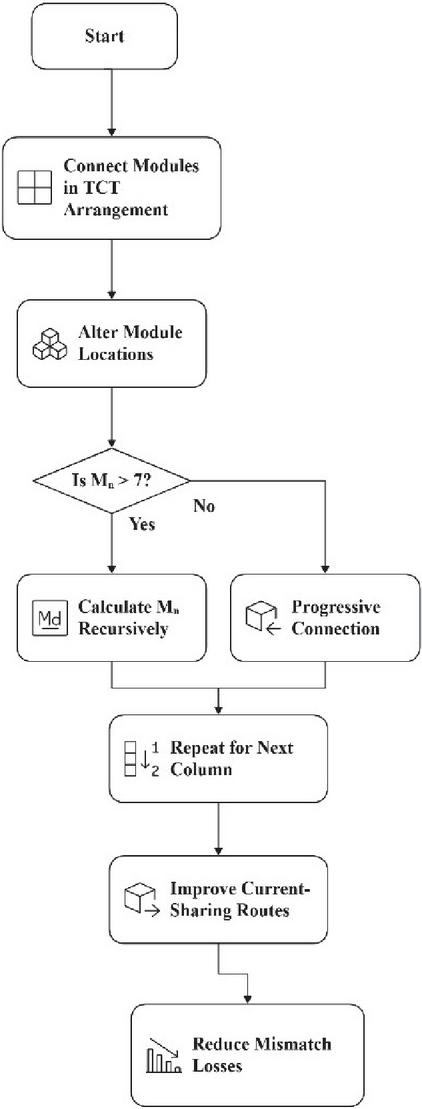
Figure 2 Process diagram of the dispersed illumination technique.

In the same way, M₁ $=$ m $+$ 2 is the first number in the third column, followed by M₂ $=$ M${}_1{}^{}+1$, M₃ $=$ M${}_2{}^{}+1$, and so on, until M₅ $=$ M${}_4{}^{}+1$ (until M${}_{\mathrm{n}}{}^{}=7$). The same alternating rule, where M₆ $=$ M₅ $-$ M₄ and M₇ $=$ M${}_6{}^{}+1$, is used when M${}_{\mathrm{n}}{}^{}>7$. For every additional column, this process is repeated in an analogous manner, with the initial offset rising by one. As a result, the TCT configuration-derived modules are systematically rearranged spatially by the Dispersed Illumination structure, improving current-sharing routes and significantly lowering mismatch losses under non-uniform irradiance.

The proposed technique’s logical structure is illustrated in Figure 2. Every step, from data entry to final configuration, demonstrates how the algorithm methodically improves the module current uniformity.

4 Case Studies for Different Shading Patterns

Beyond physical configuration methods, electrical reconfiguration strategies have also been created to adjust electrical connections dynamically according to shading conditions, aiming to spread the impact of shade across the PV array. However, the complexity of the system and the expense of hardware implementation rise due to the large quantity of voltage and current sensors needed for these methods. This paper proposes a reconfiguration that can spread the shading effect without altering the electrical connections.

The row current of modules for various illuminations is provided by:

$$I_i=\sum _j^t{k}_n{S}_n{I}_m$$

Where, $Im$ is the module current under normal operating conditions, Sn is the shade percentage at nth illumination level, $kn$ is the number of modules receiving $n$th illumination level, and n is the various illumination levels.

Taking different illuminations of various intensities,

Case Study I: In this pattern the shaded rows and column can be seen from the Figure 3 the majority of the rows are not shaded. Determine the current passing through each PV array row in order to calculate the value of global maxima.

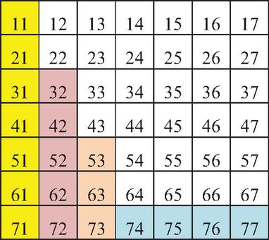
Figure 3 TCT configuration for Case I shading.

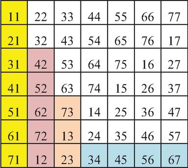
Figure 4 Dispersed illumination configuration for Case I shading.

For Case I, the row currents of the TCT, Odd–Even and DIT configured PV array are calculated based on the irradiance distribution across each module and is calculated as:

For TCT configuration In row 1 and 2, one panel receive 200 W/m² while the remaining panels are subjected to 1000 W/m²

$${\mathrm{I}}_{\mathrm{R1}}={\mathrm{I}}_{\mathrm{R2}}=6\times 1.0{\mathrm{I}}_{\mathrm{m}}+1\times 0.2{\mathrm{I}}_{\mathrm{m}}=6.2{\mathrm{I}}_{\mathrm{m}}$$

Similarly,

${\mathrm{I}}_{\mathrm{R3}}={\mathrm{I}}_{\mathrm{R4}}=5\times 1.0{\mathrm{I}}_{\mathrm{m}}+1\times 0.2{\mathrm{I}}_{\mathrm{m}}+1\times 0.3{\mathrm{I}}_{\mathrm{m}}=5.5{\mathrm{I}}_{\mathrm{m}}$

${\mathrm{I}}_{\mathrm{R5}}={\mathrm{I}}_{\mathrm{R6}}=4\times 1.0{\mathrm{I}}_{\mathrm{m}}+1\times 0.2{\mathrm{I}}_{\mathrm{m}}+1\times 0.3{\mathrm{I}}_{\mathrm{m}}+1\times 0.5{\mathrm{I}}_{\mathrm{m}}=5.0{\mathrm{I}}_{\mathrm{m}}$

${\mathrm{I}}_{\mathrm{R7}}=4\times 0.7{\mathrm{I}}_{\mathrm{m}}+1\times 0.5{\mathrm{I}}_{\mathrm{m}}+1\times 0.3{\mathrm{I}}_{\mathrm{m}}+1\times 0.2{\mathrm{I}}_{\mathrm{m}}=3.8{\mathrm{I}}_{\mathrm{m}}$

For Odd–Even

${\mathrm{I}}_{\mathrm{R1}}=1\times 0.2{\mathrm{I}}_{\mathrm{m}}+6\times 1.0{\mathrm{I}}_{\mathrm{m}}=6.2{\mathrm{I}}_{\mathrm{m}}$

${\mathrm{I}}_{\mathrm{R2}}=1\times 0.5{\mathrm{I}}_{\mathrm{m}}+6\times 1.0{\mathrm{I}}_{\mathrm{m}}=6.5{\mathrm{I}}_{\mathrm{m}}$

${\mathrm{I}}_{\mathrm{R3}}={\mathrm{I}}_{\mathrm{R4}}=3\times 1.0{\mathrm{I}}_{\mathrm{m}}+1\times 0.4{\mathrm{I}}_{\mathrm{m}}+1\times 0.3{\mathrm{I}}_{\mathrm{m}}+1\times 0.5{\mathrm{I}}_{\mathrm{m}}=4.2{\mathrm{I}}_{\mathrm{m}}$

${\mathrm{I}}_{\mathrm{R5}}=7\times 1.0{\mathrm{I}}_{\mathrm{m}}=7.0{\mathrm{I}}_{\mathrm{m}}$

${\mathrm{I}}_{\mathrm{R6}}=4\times 0.7{\mathrm{I}}_{\mathrm{m}}+1\times 0.3{\mathrm{I}}_{\mathrm{m}}+2\times 1.0{\mathrm{I}}_{\mathrm{m}}=5.1{\mathrm{I}}_{\mathrm{m}}$

${\mathrm{I}}_{\mathrm{R7}}=1\times 1.0{\mathrm{I}}_{\mathrm{m}}+1\times 0.4{\mathrm{I}}_{\mathrm{m}}+1\times 0.6{\mathrm{I}}_{\mathrm{m}}=4.0{\mathrm{I}}_{\mathrm{m}}$

For DI Technique

${\mathrm{I}}_{\mathrm{R1}}={\mathrm{I}}_{\mathrm{R7}}=4\times 1.0{\mathrm{I}}_{\mathrm{m}}+1\times 0.2{\mathrm{I}}_{\mathrm{m}}+1\times 0.3{\mathrm{I}}_{\mathrm{m}}+1\times 0.5{\mathrm{I}}_{\mathrm{m}}=5.0{\mathrm{I}}_{\mathrm{m}}$

${\mathrm{I}}_{\mathrm{R2}}=5\times 1.0{\mathrm{I}}_{\mathrm{m}}+1\times 0.2{\mathrm{I}}_{\mathrm{m}}+1\times 0.5{\mathrm{I}}_{\mathrm{m}}=5.7{\mathrm{I}}_{\mathrm{m}}$

${\mathrm{I}}_{\mathrm{R3}}=5\times 1.0{\mathrm{I}}_{\mathrm{m}}+1\times 0.2{\mathrm{I}}_{\mathrm{m}}+1\times 0.7{\mathrm{I}}_{\mathrm{m}}=5.9{\mathrm{I}}_{\mathrm{m}}$

${\mathrm{I}}_{\mathrm{R4}}={\mathrm{I}}_{\mathrm{R5}}={\mathrm{I}}_{\mathrm{R6}}=4\times 1.0{\mathrm{I}}_{\mathrm{m}}+1\times 0.2{\mathrm{I}}_{\mathrm{m}}+1\times 0.3{\mathrm{I}}_{\mathrm{m}}+1\times 0.7{\mathrm{I}}_{\mathrm{m}}$

$=5.2I_m$

The same calculation procedure is applied to the remaining four cases.

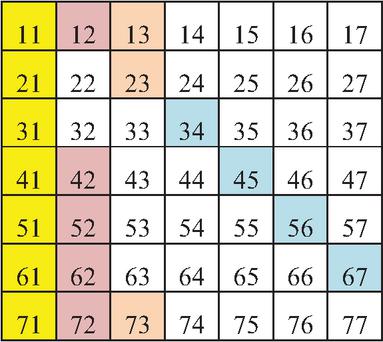
Figure 5 Shade diffusion by dispersed illumination configuration for Case I shading.

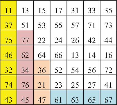
Figure 6 Odd–Even configuration for Case I shading.

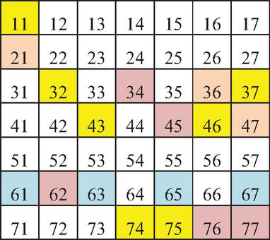
Figure 7 Shade diffusion by odd-even configuration for Case I shading.

Table 1 presents the TCT, Odd–Even and DIT configured PV array findings for Case I. It provides the voltage and current for the module in the configuration depicted in Case I. Table 1 indicates that the generated current in each row varies.

Table 1 Location of GM in TCT, DIT and Odd–Even configurations

Technique	Order	Current (Im)	Voltage (Vm)	Power (VmIm)
TCT	IR7	3.8	7	26.6
	IR6	5.0	6	30.0
	IR5	5.0	6	30.0
	IR4	5.5	5	27.5
	IR3	5.5	5	27.5
	IR2	6.2	4	24.8
	IR1	6.2	4	24.8
DIT	IR7	5.0	7	35.0
	IR1	5.0	7	35.0
	IR6	5.2	6	31.2
	IR5	5.2	6	31.2
	IR4	5.2	6	31.2
	IR2	5.7	5	28.5
	IR3	5.9	4	23.6
Odd–Even	IR7	4.0	7	28.0
	IR3	4.2	6	25.2
	IR4	4.2	6	25.2
	IR6	5.1	5	25.5
	IR1	6.2	4	24.8
	IR2	6.5	3	19.5
	IR5	7.0	2	14.0

Case Study II: Only the last three rows and first two columns are under shade in this design; the majority of the rows are not. Ascertain the current passing through each PV array row in order to calculate the value of the global maxima. Use the same calculating formula as in Case I for this.

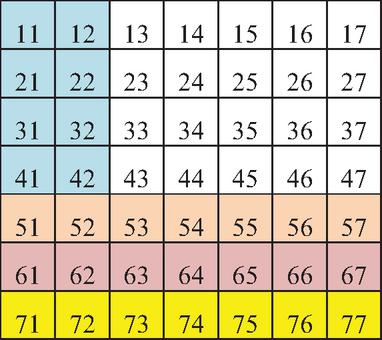
Figure 8 TCT configuration for Case II shading.

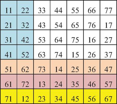
Figure 9 Dispersed illumination configuration for Case II shading.

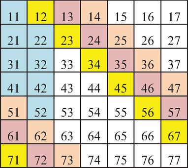
Figure 10 Shade diffusion by dispersed illumination configuration for Case II shading.

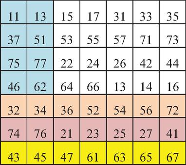
Figure 11 Odd–Even configuration for Case II shading.

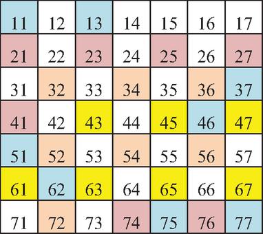
Figure 12 Shade diffusion by odd-even configuration for Case II shading.

Table 2 provides the voltage and current of the module for the configuration shown in Case II, as well as the results of the TCT, DIT and Odd–Even setup PV array. When compared to both the TCT and Odd–Even configurations, the DI setup generates a higher power output. Under the same operating conditions, the DI setup performs better even though the TCT and Odd–Even approaches outperform the traditional structure.

Table 2 Location of GM in TCT, DIT and Odd–Even configurations

Technique	Order	Current (Im)	Voltage (Vm)	Power (VmIm)
TCT	IR7	1.4	7	9.8
	IR6	2.1	6	12.6
	IR5	3.5	5	17.5
	IR4	6.4	4	25.6
	IR3	6.4	4	25.6
	IR2	6.4	4	25.6
	IR1	6.4	4	25.6
DIT	IR4	4.4	7	30.8
	IR3	4.4	7	30.8
	IR2	4.4	7	30.8
	IR1	4.7	6	28.2
	IR5	4.7	6	28.2
	IR7	5.0	5	25.0
	IR6	5.0	5	25.0
Odd–Even	IR6	3.5	7	24.5
	IR4	3.6	6	21.6
	IR2	4.2	5	21.0
	IR7	4.5	4	18.0
	IR5	5.2	3	15.6
	IR3	5.2	3	15.6
	IR1	6.4	2	12.8

Case Study III: In this specific configuration the last three rows are under shade leaving the bulk of the rows unshaded. Each PV array row’s current contribution must be examined in order to precisely calculate the global maximum power point. This can be accomplished by using the same mathematical technique that was used to calculate power and current in Case I. This method can be used to determine the exact operating point that corresponds to the global maximum and efficiently evaluate the impact of partial shade on the PV system’s overall performance.

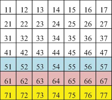
Figure 13 TCT configuration for Case III shading.

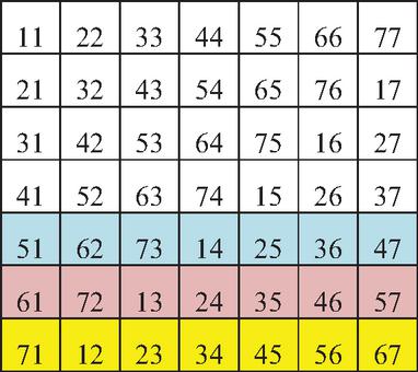
Figure 14 Dispersed illumination configuration for Case III shading.

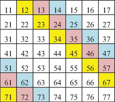
Figure 15 Shade diffusion by dispersed illumination configuration for Case III shading.

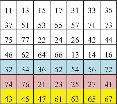
Figure 16 Odd–Even configuration for Case III shading.

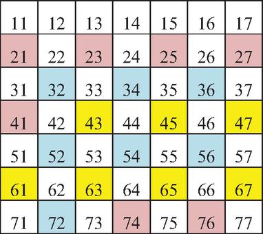
Figure 17 Shade diffusion by odd-even configuration for Case III shading.

In addition to the results of the TCT, Odd–Even and DI setup PV array, Table 3. provides the voltage and current of the module for the configuration displayed in Case III. It suggests that each row’s generated current varies.

Table 3 Location of GM in TCT, DIT and Odd–Even configurations

Technique	Order	Current (Im)	Voltage (Vm)	Power (VmIm)
TCT	IR7	1.4	7	9.8
	IR6	2.1	6	12.6
	IR5	4.9	5	24.5
	IR4	7.0	4	28.0
	IR3	7.0	4	28.0
	IR2	7.0	4	28.0
	IR1	7.0	4	28.0
DIT	IR7	5.2	7	36.4
	IR6	5.2	7	36.4
	IR5	5.2	7	36.4
	IR4	5.2	7	36.4
	IR3	5.2	7	36.4
	IR2	5.2	7	36.4
	IR1	5.2	7	36.4
Odd–Even	IR6	3.8	7	26.6
	IR4	3.9	6	23.4
	IR2	4.2	5	21.0
	IR7	5.3	4	21.2
	IR3	6.1	3	18.3
	IR5	6.1	3	18.3
	IR1	7.0	2	14.0

Case Study IV: In this shading pattern, last four rows are under shade. To determine the value of global maxima the current flowing via each PV array row must be determined using the same formula suggested in Case I for calculations.

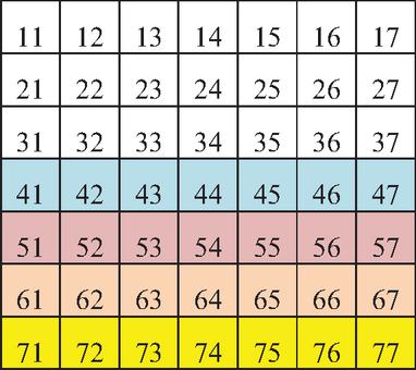
Figure 18 TCT configuration for Case IV shading.

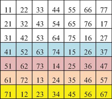
Figure 19 Dispersed illumination configuration for Case IV shading.

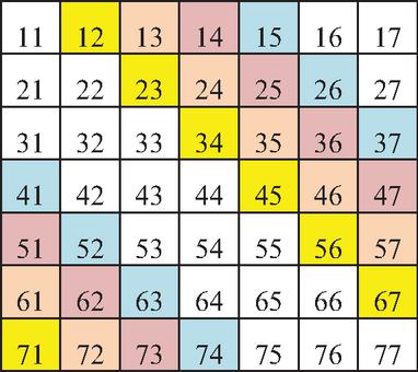
Figure 20 Shade diffusion by dispersed illumination configuration for Case IV shading.

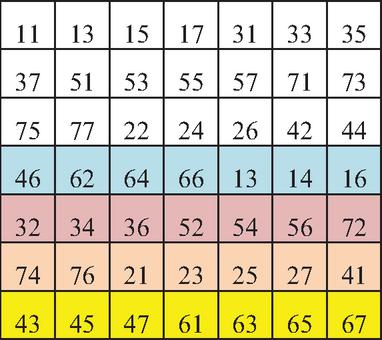
Figure 21 Odd–Even configuration for Case IV shading.

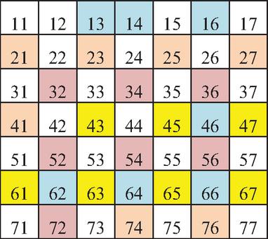
Figure 22 Shade diffusion by Odd–Even configuration for Case IV shading.

Table 4 indicates the voltage and current of the module for the configuration shown in Case IV, as well as the results of the TCT, Odd–Even and DI setup PV array.

Table 4 Location of GM in TCT, DIT and Odd–Even configurations

Technique	Order	Current (Im)	Voltage (Vm)	Power (VmIm)
TCT	IR7	1.4	7	9.8
	IR5	2.1	6	12.6
	IR6	3.5	5	17.5
	IR4	4.9	4	19.6
	IR3	7.0	3	21.0
	IR2	7.0	3	21.0
	IR1	7.0	3	21.0
DIT	IR7	4.7	7	32.9
	IR1	4.7	7	32.9
	IR6	4.7	7	32.9
	IR5	4.7	7	32.9
	IR4	4.7	7	32.9
	IR2	4.7	7	32.9
	IR3	4.7	7	32.9
Odd–Even	IR6	2.9	7	20.3
	IR4	3.6	6	21.6
	IR5	4.9	5	24.5
	IR3	4.9	5	24.5
	IR2	5.0	4	20.0
	IR7	5.3	3	15.9
	IR1	6.1	2	12.2

Case Study V: In this configuration the rows and columns are under shade in such a way that the shade resembles a square shape which can be seen from Figure 23 leaving the bulk of the rows unshaded. Each PV array row’s current contribution must be examined in order to precisely calculate the global maximum power point. This can be accomplished by using the same mathematical technique that was used to calculate power and current in Case I. By using this method, the exact operating point that corresponds to the global maximum and efficiently evaluate the impact of partial shade on the PV system’s overall performance.

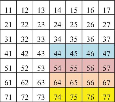
Figure 23 TCT configuration for Case V shading.

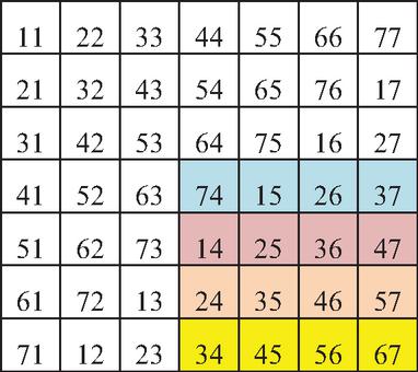
Figure 24 Dispersed illumination configuration for Case V shading.

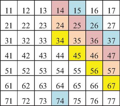
Figure 25 Shade diffusion by dispersed illumination configuration for Case V shading.

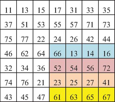
Figure 26 Odd–Even configuration for Case V shading.

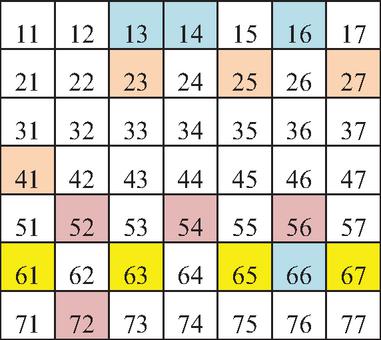
Figure 27 Shade diffusion by Odd–Even configuration for Case V shading.

Table 5 Location of GM in TCT, DIT and Odd–Even configurations

Technique	Order	Current (Im)	Voltage (Vm)	Power (VmIm)
TCT	IR7	3.8	7	26.6
	IR5	4.2	6	25.2
	IR6	5.0	5	25.0
	IR4	5.8	4	23.2
	IR3	7.0	3	21.0
	IR2	7.0	3	21.0
	IR1	7.0	3	21.0
DIT	IR3	4.7	7	32.9
	IR4	5.0	6	30.0
	IR2	5.5	5	27.5
	IR5	5.7	4	22.8
	IR1	6.0	3	18.0
	IR6	6.2	2	12.4
	IR7	6.7	1	6.7
Odd–Even	IR6	3.5	7	24.5
	IR5	4.9	6	29.4
	IR2	5.5	5	27.5
	IR1	6.1	4	24.4
	IR7	6.3	3	18.9
	IR4	6.5	2	13.0
	IR3	7.0	1	7.0

Table 5 provide the module’s voltage and current for the setup depicted in Case V along with the outcomes of the PV array’s TCT, DI and Odd–Even setup.

5 Results and Discussion

The P-V characteristics of the PV system under various shading conditions using DIT and TCT methodologies are depicted in the following figures, which correspond to Cases I to V respectively. Because of the shading effect, several local maxima can be observed in every instance. In many situations, the TCT approach has a tendency to converge around local peaks, which results in lower power production and observable oscillations. The DIT approach, on the other hand, reliably locates and monitors the global maximum power point (GMPP), providing more constant and higher power under all shading conditions.

Overall, the findings show that under several kinds of partial shading conditions, the DIT approach offers better tracking accuracy, increased stability, and improved power extraction performance.

Table 6 provides a summary of the essential electrical parameters for each case. Under various partial shade situations, the table illustrates the maximum power (P_max), maximum voltage (V_max), open-circuit voltage (V_oc), and short-circuit current (I_sc) for both TCT and the suggested DIT approach. The PV array power comparison for TCT, Odd–Even, and the suggested method under various partial shading conditions is shown case-by-case in Table 7. When compared to TCT and Odd–Even arrangements, it is evident that the suggested method consistently produces the highest power production. Although the TCT and Odd–Even approaches exhibit lower power because of shading-induced mismatch losses, the suggested method significantly boosts the extracted power, proving its efficacy in reducing mismatch losses and enhancing system performance.

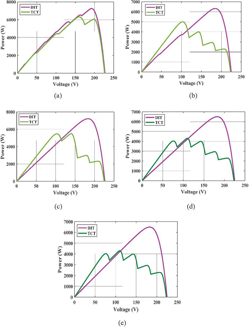
Figure 28 Comparative P-V curves of the PV array under partial shading conditions for different cases.

Table 6 Output performance parameters of PV array for various operating cases

Configurations		Pmax(W)	Vmax(V)	Voc (V)	Isc(A)
Case I	TCT	6315	160.0	226.5	50.86
	DIT	7241	185.1	226.6	48.34
Case II	TCT	4996	102.6	223.1	52.53
	DIT	6323	184.6	225.1	41.01
Case III	TCT	5492	140.0	224.3	57.46
	DIT	7214	183.1	226.3	42.69
Case IV	TCT	4303	110.0	223.4	57.45
	DIT	6497	182.7	224.9	38.59
Case V	TCT	6078	199.0	227.1	57.45
	DIT	7258	192.6	227.3	54.91

Table 7 Case wise power output comparison of PV array configurations

Cases	TCT	Odd Even	Proposed Technique
CASE I	6315W	4962W	7241W
CASE II	4996W	4902W	6323W
CASE III	5492W	5322W	7214W
CASE IV	4303W	4902W	6497W
CASE V	6078W	5883W	7258W

Table 8 Performance comparison of TCT and DI based on mismatch and shading losses

	Shading Cases
	Case I		Case II		Case III		Case IV		Case V
Parameters	TCT	DI	TCT	DI	TCT	DI	TCT	DI	TCT	DI
Pmax(W)	7440	7440	6520	6520	7280	7280	6580	6580	7960	7960
Pact(W)	6315	7241	4996	6323	5492	7214	4303	6497	6078	7258
P${}_{\text{max’s}}$(W)	9800	9800	9800	9800	9800	9800	9800	9800	9800	9800
Voc(V)	226.5	226.6	223.1	225.1	224.3	226.3	223.4	224.9	227.1	227.3
Isc(A)	50.86	48.34	52.53	41.01	57.46	42.69	57.45	38.59	57.45	54.91
PML(W)	1125	199.0	1524	197.0	1788	66.00	2277	83.00	1882	702.0
PSL(W)	2360	2360	3280	3280	2520	2520	3220	3220	1840	1840
FF	0.548	0.661	0.426	0.685	0.426	0.746	0.335	0.573	0.465	0.581

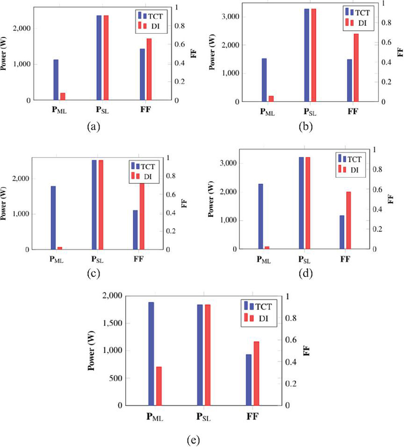
Figure 29 P_ML, P_SL, and FF comparison between TCT and DI configurations for Cases I–V under partial shading conditions.

6 Comparison of Losses and Fill Factor

6.1 Losses Comparison

The TCT, DIT, and Odd–Even PV array topologies are taken into consideration for the comparative analysis. Under the chosen shading conditions, a thorough analysis is conducted on these three configurations to look at their electrical properties, power output behaviour, and loss distribution. A methodical evaluation of their performance in terms of mismatch loss reduction, effect on shading losses and power augmentation capability under partial shade conditions is made easier by this comparison.

(A) Mismatch loss: It is defined as the difference between the sum of the maximum power outputs of individual panels under a specific mismatch or shading conditions ($P_{\mathit{max}}$), to the actual peak power output of the PV array ($P_{\mathit{act}}$). Equation (5) is used to compute the mismatch loss. This formula is used to figure out and show the mismatch losses in Table 8, and Figure 29 provides a visual comparison of several PV array layouts. When assessing PV array topologies under different partial shade conditions (PSCs), mismatch loss is a crucial performance parameter. Various array layouts encourage row current equalization, which reduces the shading effect. A decrease in mismatch losses suggests that the PV array arrangement is more effective and performs better.

$${\mathrm{P}}_{\mathrm{ML}}={\mathrm{P}}_{\max }-{\mathrm{P}}_{\mathrm{act}}$$

(5)

(B) Shading loss: It is the defined as the difference between the PV array’s optimal power output under standard operating conditions ($P_{\text{max’s}}$) and the peak power output of each panel under mismatch or partial shading conditions ($P_{\mathit{max}}$) and it is represented by Equation (6). The shading losses are computed using Equation (6) and shown in Table 8. As partial shade occurs in real-world PV installations, shading losses are unavoidable. The magnitude of the shading effect on system performance can be seen by these losses. Each of the variations have the same peak power under standard insolation conditions. Similarly, the algebraic sum of the PV array’s individual panels’ peak power outputs for a certain shading pattern is the same for all layouts.

$${\mathrm{P}}_{\mathrm{SL}}={\mathrm{P}}_{\text{max’s}}-{\mathrm{P}}_{\max }$$

(6)

6.2 Fill Factor

The quality or squareness of a PV array’s I-V characteristics is indicated by the fill factor. Its value should ideally equal unity, which would represent a perfect rectangular I-V curve. The practical I-V characteristics near to the ideal situation is shown by the fill factor. It is described by the open-circuit voltage ($V_{\mathit{oc}}$), the short-circuit current ($I_{\mathit{sc}}$), and the maximum power at the global maximum power point ($P_{\mathit{GMPP}}$) for every instance of partial shade or mismatch.

$$\mathrm{FF}=\frac{\mathrm{PGMPP}}{\mathrm{Voc}\times \mathrm{Isc}}$$

(7)

The fill factor is determined using Equation (7) and shown in Table 8. Figure 29 provides a further graphic representation of a comparative analysis of the fill factor for several PV array layouts.

7 Conclusion

The DI technique is presented in this study under five distinct PV array partial shading conditions. This method increases an array’s generating power. The findings of the DI technique also compared with TCT technique and Odd–Even under different partial shading conditions and it was shown that DI technique generates greater power output under same partial shading conditions. This suggested method also lowers several peaks in the power voltage characteristics.

The performance of the proposed DI technique is evaluated under five distinct partial shading conditions, as summarized below:

• The TCT-configured PV array in Case I generates 6315 W of output power. When the DIT arrangement is implemented, the output power increases significantly to 7241 W, whereas the Odd–Even configuration results in a lesser output of 4962 W.

• In Case II, the PV array’s maximum power production under the TCT arrangement is 4996 W. When the DIT arrangement is used, this value rises to 6323 W, while the Odd–Even configuration has a power output of 4902 W.

• The PV array set up in TCT configuration in Case III has a maximum power output of 5492 W. The output power rises significantly to 7214 W when the DIT configuration is used. The Odd–Even design, on the other hand, produces a significantly lower power rating of 5322 W.

• In Case IV, the TCT configuration produces a much lower output of 4303 W, while the DIT configured PV array has a maximum power output of 6497 W. This suggests that the DIT arrangement improves power extraction and reduces power loss, resulting in increased energy extraction, whereas the power output of the Odd–Even arrangement is 4902 W.

• In Case V, a maximum power output of 6078 W is produced by the PV array using the TCT arrangement. The output power rises to 7258 W when the DIT configuration is used, showing better performance. In comparison, the Odd–Even arrangement results in a maximum power output of 5883 W.

References

[1] R. K. Pachauri et al., “Impact of Partial Shading on Various PV Array Configurations and Different Modeling Approaches: A Comprehensive Review,” in IEEE Access, vol. 8, pp. 181375–181403, 2020, doi:10.1109/ACCESS.2020.3028473.

[2] Mohd Faisal Jalil, Dushyant Sharma, R.C. Bansal, Cross kit reconfiguration algorithm for enhanced output power of PV array during shading mismatch conditions, Optik, Volume 288, 2023, 171218, https://doi.org/10.1016/j.ijleo.2023.171218.

[3] Okan Bingöl, Burçin Özkaya, Analysis and comparison of different PV array configurations under partial shading conditions, Solar Energy, Volume 1602018, ISSN 0038092X, https://doi.org/10.1016/j.solener.2017.12.004.

[4] Ibraheem Nasiruddin, Shahida Khatoon, Mohd Faisal Jalil, R.C. Bansal, Shade diffusion of partial shaded PV array by using odd-even structure, Solar Energy, Volume 181, 2019 ISSN 0038092X, https://doi.org/10.1016/j.solener.2019.01.076.

[5] Iskandar, Handoko, Bakti, Zainal and Sambasri, Susanto. (2018). Study and Analysis of Shading Effects on Photovoltaic Application System. MATEC Web of Conferences. 218. 02004. doi:10.1051/matecconf/201821802004.

[6] Osmani K, Haddad A, Jaber H, et al. Mitigating the effects of partial shading on PV system’s performance through PV array reconfiguration: a review. Therm Sci Eng Prog. 2022;31:101280. doi:10.1016/J.TSEP.2022.101280.

[7] Injila Sajid, Adil Sarwar, Mohd Tariq, Farhad Ilahi Bakhsh, Shafiq Ahmad, Adamali Shah Noor Mohamed, Archimedes optimization algorithm (AOA)-Based global maximum power point tracking for a photovoltaic system under partial and complex shading conditions, Energy, Volume 283, 2023, 129169, ISSN 0360-5442, https://doi.org/10.1016/j.energy.2023.129169.

[8] Mohd Faisal Jalil, Shahida Khatoon, Rahma Aman, Salman Hameed and R.C. Bansal (2023) Alternate panel interchange technique to improve the power production of PV array operating under various shading situations, International Journal of Modelling and Simulation, 43:6, 849–863, doi:10.1080/02286203.2022.2127054.

[9] Anjum S, Mukherjee V. Static and dynamic reconfiguration strategies for reducing partial shading effects in photovoltaic array: a comprehensive review. Energy Technol. 2022;10(7):2200098. doi:10.1002/ENTE.202200098.

[10] G. Sai Krishna, Tukaram Moger, Reconfiguration strategies for reducing partial shading effects in photovoltaic arrays: State of the art, Solar Energy, Volume 182, 2019, https://doi.org/10.1016/j.solener.2019.02.057.

[11] Verma, P., Alam, A., Sarwar, A., Tariq, M., Vahedi, H., Gupta, D.: Meta-heuristic optimization techniques used for maximum power point tracking in solar PV system. Electronics 10, 2021 (2419).

[12] Lamprini Papargyri, Marios Theristis, Bernhard Kubicek, Thomas Krametz, Christoph Mayr, Panos Papanastasiou, George E. Georghiou, Modelling and experimental investigations of microcracks in crystalline silicon photovoltaics: A review, Renewable Energy, Volume 145, 2020, Pages 2387-2408, ISSN 0960-1481, https://doi.org/10.1016/j.renene.2019.07.138.

[13] Sajid, I., Sarwar, A., Tariq, M., Ahmad, S., Bakhsh, F.I., Mohamed, A.S.N., Islam, M.R.: An MPPT method using phasor particle swarm optimization for PV-based generation system under varying irradiance conditions. IET Renew. Power Gener. 18, 4197–4209 (2024). https://doi.org/10.1049/rpg2.13158.

[14] Jour, Rezazadeh, Sevda, Moradzadeh, Arash, Pourhossein, Kazem, Mohammadi-Ivatloo, Behnam, Garc�a Márquez, Fausto Pedro, 2023, 2023/09/01, Photovoltaic array reconfiguration under partial shading conditions for maximum power extraction via knight’s tour technique, https://doi.org/10.1007/s12652-022-03723-1.

[15] Gautam, V., Khatoon, S., Jalil, M. F., & Bansal, R. C. (2024). Comparative analysis of various reconfiguration strategies of PV array in partial shading conditions: a review. International Journal of Modelling and Simulation, 1–34. https://doi.org/10.1080/02286203.2024.2403008.

[16] Vandana Jha, Generalized modelling of PV module and different PV array configurations under partial shading condition, Sustainable Energy Technologies and Assessments, Volume 56, 2023, 103021, ISSN 2213-1388, https://doi.org/10.1016/j.seta.2023.103021.

[17] Kour J, Shukla A. Comparative analysis of different reconfiguration schemes for power enhancement under various shading scenarios. Sol Energy. 2021;230:91–108. doi:10.1016/J.SOLENER.2021.10.001.

[18] Nassef AM, Houssein EH, Din Helmy BE, et al. Optimal reconfiguration strategy based on modified Runge Kutta optimizer to mitigate partial shading condition in photovoltaic systems. Energy Rep. 2022;8:7242–7262. doi:10.1016/J.EGYR.2022.05.231.

[19] Shahroz Anjum, V. Mukherjee, Gitanjali Mehta, Modelling and simulation of AdDoKu based reconfiguration technique to harvest maximum power from photovoltaic array under partial shading conditions, Simulation Modelling Practice and Theory, Volume 115, 2022, 102447, ISSN 1569-190X, https://doi.org/10.1016/j.simpat.2021.102447.

[20] Anurag Singh Yadav, V. Mukherjee, Conventional and advanced PV array configurations to extract maximum power under partial shading conditions: A review, Renewable Energy, Volume 178, 2021, Pages 977–1005, ISSN 0960-1481, https://doi.org/10.1016/j.renene.2021.06.029.

[21] Rani, B., Ilango, G. and Chilakapati, Nagamani. (2013). Enhanced Power Generation from PV Array Under Partial Shading Conditions by Shade Dispersion Using Su Do Ku Configuration. Sustainable Energy, IEEE Transactions on. 4. 594–601. doi:10.1109/TSTE.2012.2230033.

[22] Chidurala Saiprakash, Alivarani Mohapatra, Byamakesh Nayak, Sriparna Roy Ghatak, Analysis of partial shading effect on energy output of different solar PV array configurations, https://doi.org/10.1016/j.matpr.2020.08.307.

[23] Villalva MG, Gazoli JR, Filho ER. Comprehensive approach to modeling and simulation of photovoltaic arrays. IEEE Trans Power Electron. 2009;24(5):1198–1208.

Biographies

AL Shifa Kafeel is a final year student of Electrical Engineering at Zakir Husain College of Engineering and Technology, Aligarh Muslim University. She has strong interest in renewable energy especially solar energy generation, and has research experience in the field and has published a conference paper. Along with having a strong academic background, she is also an active member of the IEEE community being Vice Chairperson of the IEEE STB, AMU. She also has an offer to join as GET at Larsen & Toubro.

Zeeshan Ali Khan is a final-year undergraduate student pursuing a Bachelor’s degree in Electrical Engineering at Zakir Husain College of Engineering and Technology, Aligarh Muslim University (AMU), Aligarh, India. He has worked as a Research Intern at the APJ Abdul Kalam STEM-ER Centre (Indo–US collaboration), AMU. His research interests include power electronics, renewable energy systems, battery management.

Mohd Faisal Jalil has more than 14 years of teaching and research experience. He is a Senior Member of IEEE. Currently, he is working as an Assistant Professor in the Electrical Engineering department, Aligarh Muslim University, Aligarh, India. He has published several research papers in reputed journals and conferences. His research interests include electrical machines, renewable energy systems, and PV systems under partial shading conditions.

Strategic Planning for Energy and the Environment, Vol. 45_3, 977–1006
doi: 10.13052/spee1048-5236.45313
© 2026 River Publishers