Capacity Adequacy Performance Payment Strategy Considering Seasonal Fluctuations of Hydropower
Wei Guangxu* and Dong Shuo
Northeast Electric Power University, School of Electrical Engineering, Jilin, China
E-mail: weiguangxu25@163.com
*Corresponding Author
Received 16 February 2026; Accepted 15 April 2026
Abstract
The long-term stable adequacy of power generation capacity and flexible adjustable resources is one of the keys to the stable operation of the power market. The uncertainty of new energy and the periodicity of hydropower output pose greater challenges to the adequacy of power market capacity and adjustable resources. To address this challenge, probabilistic modeling of error probabilities in different periods is conducted through the kernel density estimation method with separate parameters. Dynamic reserve capacity demand is calculated under confidence probability, and capacity adequacy performance payment is introduced. Finally, the incentive effects of the new method are compared with those of the traditional capacity payment system and market auction in the market, leading to the conclusion that the new method helps flexible adjustable units better recover costs.
Keywords: Seasonal capacity, capacity market, reserve capacity, kernel density estimation, performance payment.
1 Introduction
Driven by the green transformation of the energy structure and the “dual carbon” goals, the installed capacity of new energy has grown rapidly. Its intermittency and volatility have increased the pressure on the safe and stable operation of the power system. Yunnan Province has long relied on hydropower, with hydropower accounting for 71.23% of the province’s total electricity consumption in 2024. However, the declining economics of thermal power units have weakened the investment attractiveness of coal-fired units, leading to stagnant growth in installed capacity. Due to the seasonal fluctuations of run-of-river hydropower and insufficient installed capacity of coal-fired units in Yunnan Province, there is a shortage of flexible and adjustable resources during the dry season of hydropower.
Under the current power market system, thermal power units face problems such as high capital investment, long investment return cycles, limited profitability, and declining investment willingness of market participants [1, 2]. In Yunnan Province, run-of-river hydropower generates a large amount of electricity during the wet season, and due to its relative stability, the demand for flexible and adjustable resources is relatively small during this period. However, during the dry season, hydropower generation drops sharply, while the output of renewable energy such as wind and solar power increases, bringing significant uncertainty to the power system [3] and a sharp rise in the demand for flexible capacity [4]. Nevertheless, the traditional capacity compensation methods in various regions have not fully reflected the value of this part of flexible and adjustable capacity, which further inhibits the investment willingness of adjustable units during the dry season, exacerbates the supply-demand gap, and forms a vicious circle. With the development of the power market, the peak shaving auxiliary service market has also brought certain positive incentives for capacity investment to a certain extent. However, studies have pointed out that the current revenue from auxiliary service markets such as peak shaving is not sufficient to offset the actual losses of units [5, 6].
Based on the above problems, the power market needs new market mechanisms that can not only alleviate the current decline in investment willingness of thermal power units but also comprehensively consider the energy background to provide effective market signals to reflect the actual value of power generation capacity and flexible adjustable capacity during scarce periods. In 2023, China also began to subsidize relevant flexible capacity with fixed-amount subsidies [7], transitioning towards a “two-part” electricity price mechanism.
At present, traditional capacity compensation methods are mainly divided into two types. The first type can be collectively referred to as the capacity payment mechanism [8–10]. The systems vary greatly among different countries and regions, but the core idea is generally to provide payment subsidies for specific required capacity to increase the revenue of the required capacity and provide positive market incentives. The second type is the capacity market [11–14]. Recent studies highlight the value of emerging entities like energy storage and virtual power plants. Tailored market mechanisms can effectively incentivize their participation and significantly reduce system reserve costs [15]. capacity and tiered tariffs secure the grid but constrain the optimal PV capacity in distribution networks [16]. a multi-agent model based on the Deep Deterministic Policy Gradient (DDPG) algorithm was established. This study utilized deep reinforcement learning to model and simulate the complex bidding behaviors of power generation enterprises within the market [17]. The power market predicts future power generation capacity demand through market prices from bilateral transactions and centralized auctions. Power generation enterprises provide capacity products to obtain capacity fees, thereby recovering part of the fixed costs.
Although capacity payment mechanisms vary greatly among different countries and regions, their overall ideas are similar and have certain positive effects. However, they rely heavily on the system design of regulatory authorities, with low market risks but economic efficiency related to the subsidy amount designed by the authorities, which is quite difficult to design. The capacity market method has made certain explorations in optimizing capacity prices, but both methods still have certain limitations in addressing the shortage of flexible and adjustable capacity during the dry season in regions rich in hydropower resources.
This paper first introduces the two traditional market mechanisms by taking the capacity payment system and capacity market auction in Yunnan region and the United States PJM as examples. Then, aiming at the problems raised above and comprehensively considering the energy background, it conducts probabilistic modeling of error probabilities in different periods through the kernel density estimation method of parameter distribution, calculates dynamic reserve capacity demand under confidence probability, and introduces capacity adequacy performance payment. Finally, it compares the incentive effects of the new method with the traditional capacity payment system and market auction in the market.
2 Monthly Auction Model
Auction clearing is essentially an optimization problem balancing economic efficiency and reliability. Without considering economic efficiency, increasing capacity will naturally improve system stability, since a more abundant capacity corresponds to a higher system reliability. However, from an economic perspective, it is always necessary to find a balance between economic efficiency and reliability, and determining such a balance is also an economic issue [18]. The traditional view holds that the true market value of goods can be discovered through market mechanisms. Therefore, monthly auctions are held to identify the actual value of incremental capacity in power systems across different seasonal periods, and to incentivize capacity investors to independently configure reserve capacity that balances economic efficiency and reliability.
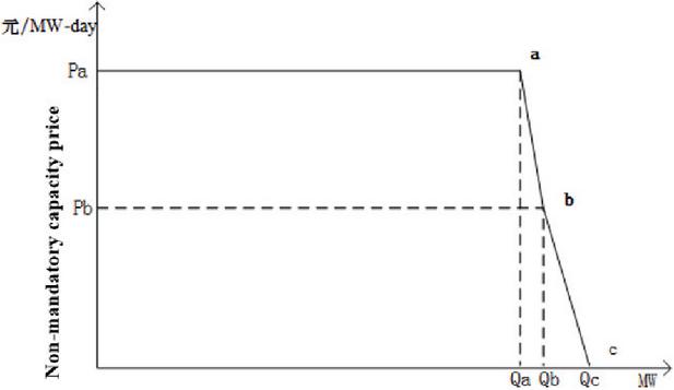
Figure 1 Capacity demand curve.
2.1 Capacity Demand for Monthly Auctions
The determination of auction capacity is usually conducted through the capacity demand curve issued by regulatory or operational institutions. For example, the PJM power market adopts the Variable Resource Requirement (VRR) curve, which has been widely applied in markets such as the US MISO power market and the New York Independent System Operator (NYISO) power market. Market operators determine the VRR curve based on parameters including the peak value of system load forecast, installed reserve margin, and the cost of newly-built generating units. Figure 1 illustrates the capacity market clearing with the VRR curve adopted. The formulation of the capacity demand curve in the subsequent research of this paper refers to the calculation method of the capacity demand curve specified in the PJM Power Market Manual [19].
The calculation formulas for the capacity and price at inflection points a, b and c of the capacity demand curve are as follows:
| (1) | |
| (2) | |
| (3) | |
| (4) | |
| (5) |
Wherein, and represent the capacity prices at inflection points a and b on the capacity demand curve, respectively; , , and denote the corresponding capacity requirement targets at inflection points a, b, and c. CONE denotes the cost of new entry, E&AS represents the revenue from the energy and ancillary services market, PE WEFORD is the market equivalent forced outage rate, RR stands for the reliability requirement coefficient, and AIRM refers to the assessed installed reserve margin.
2.2 Objective Function
In the monthly auction market, unilateral bidding is submitted by sellers (capacity owners), and market clearing is conducted based on the capacity demand curve specified by PJM. The market aims to minimize the total cost of system capacity procurement, with the objective function shown in Equation (6):
| (6) |
In the equation, denotes the clearing price of the -th thermal power unit, denotes the clearing price of the -th hydropower unit, denotes the clearing price of the -th wind power unit, and denotes the clearing price of the -th photovoltaic unit; is the bid capacity of the -th thermal power unit, is the capacity of the -th hydropower unit, is the bid capacity of the -th wind power unit, and is the bid capacity of the -th photovoltaic unit. , , and represent the sets of thermal power units, hydropower units, wind power units and photovoltaic units, respectively.
2.3 Constraints
(1) Unit Capacity Constraints
The bid capacity of a unit shall not exceed its maximum installed capacity. When accounting for forced outages such as monthly maintenance, the bid capacity constraints for units are specified as follows:
| (7) | |
| (8) | |
| (9) |
Wherein, , , , and represent the bid capacities of the i-th thermal power unit, m-th hydropower unit, n-th wind power unit, and j-th photovoltaic unit, respectively. , , , and denote the maximum installed capacities of the corresponding units. , , , and refer to the equivalent forced outage rates for each respective unit.
Considering the stable seasonal output characteristics of hydropower, the actual bid capacity shall not exceed the historical maximum power output in the same season and hydrological period in recent years, or the power generation output corresponding to predicted precipitation. That is, the bid capacity constraint for hydropower units can be optimized as follows:
| (10) |
Qy is the historical maximum power output or the power generation output corresponding to predicted precipitation of the hydropower unit in hydrological period y.
It is worth noting that the bid capacity constraints in this model implicitly incorporate the Capacity Credit of different power sources. For thermal units, Equation (7) accounts for the Equivalent Forced Outage Rate (EFORd) to reflect their mechanical reliability. For hydropower units, Equation (10) restricts the bid capacity within the historical maximum output or predicted precipitation output for the specific hydrological period, which serves as a seasonal derating factor to ensure that the cleared capacity is realistically available.
(2) Capacity Balance Constraint
The cleared capacity of the monthly auction shall be equal to the forecasted load demand and the forecasted reserve capacity margin for the target month, namely:
To account for the differences in capacity credibility, the available capacity of renewable energy is adjusted using a Capacity Credit (CC) coefficient. The capacity balance constraint in Equation (2.3) is revised as:
| (11) |
Wherein, represents the forecasted load demand for the target month, and stands for the forecasted reserve capacity margin. , and denote the Capacity Credit coefficients for the m-th hydropower unit, n-th wind power unit, and j-th photovoltaic unit, respectively.
Specifically, the capacity credit for wind and solar is determined by their respective confidence levels calculated via KDE, ensuring that the cleared capacity reflects the actual reliable contribution to the system
| (12) |
3 Capacity Performance Payment Model Considering Flexibility
3.1 Performance Payment
Performance payment refers to the practice of conducting performance evaluation on generating units available at critical moments. As shown in Figure 2, the margin of reserve capacity fluctuates with time. When the reserve capacity is about to fall below the reserve requirement, the reserve capacity demand of regional nodes is first met through the rescheduling of internal system resources. Performance payment is triggered when the reserve capacity demand cannot be satisfied by rescheduling.
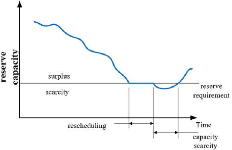
Figure 2 Performance payment.
The performance payment cycle follows a four-stage logic:
(1) Real-time Monitoring: The system operator monitors the available reserve against the dynamic reserve capacity curve.
(2) Rescheduling: If reserves are tight, internal resources are rescheduled to meet the demand.
(3) Scarcity Trigger: A scarcity event is formally triggered if the reserve requirement (defined by Equations (20) and (21)) remains unsatisfied after rescheduling.
(4) Settlement: Performance payments or penalties are calculated based on the Balancing Ratio (Br) and the Actual Capacity Provided (ACP) relative to the unit’s Capacity Supply Obligation (CSO).
At times of capacity scarcity, capacity providers that fail to fulfill their power generation obligations shall make performance payments based on the system balance ratio, the actual output of the units, and the capacity obligations they undertake in the capacity market. Meanwhile, additional payments will be granted as rewards to capacity owners who voluntarily provide extra power output. This performance payment mechanism is a relative arrangement, which is consistent with the “beneficiary pays” principle in the market and complements the capacity market. In essence, during scarcity periods, the capacity market revenues that would otherwise be generated but are lost due to the actual output falling short of the unit’s capacity obligations are converted into opportunity gains for the system. This payment method establishes an incentive mechanism that encourages suppliers to provide more stable capacity support and flexible adjustable reserve capacity, so as to meet the system’s demand for long-term capacity adequacy and address the shortage of flexible adjustable resources in certain regions. The specific calculation method for the performance payment amount is specified as follows:
| (13) |
In the equation, PP (Performance Payments) denotes the performance payment amount, PPR (Performance Payment Rate) is the performance payment rate, ACP (Actual Capacity Provided) represents the real-time available power generation capacity of the unit, Br (Balancing Ratio) stands for the balancing ratio, and CSO (Capacity Supply Obligation) refers to the capacity obligation undertaken in the monthly auction market.
The Performance Payment Rate (PPR) is the key economic incentive in this mechanism. Its value selection is based on the annualized Cost of New Entry (CONE) or the Value of Lost Load (VOLL). A reasonable range for PPR should be high enough to compensate for the opportunity costs and mechanical wear-and-tear of flexible units during deep peaking, yet remain below the regulatory price cap to prevent excessive financial risk during extreme scarcity events.
The calculation method for Br is as follows:
| (14) |
In the equation, O denotes the total capacity obligation for month m, L is the load at time t, and R represents the reserve capacity requirement at time t.
3.2 Dynamic Reserve Capacity Curve
The criterion for performance payment is the capacity demand criterion, i.e., the required reserve capacity for system operation. Traditional reserve capacity is divided into net load reserve and contingency reserve, and the maximum value of the two is generally adopted in actual operation. The net load reserve is usually 3% to 5% of the maximum load [20], while the contingency reserve is generally equivalent to the capacity of the largest generating unit in the system’s installed capacity.
However, with the continuous increase in the penetration rate of new energy, the challenges to system reserve capacity no longer stem merely from load disturbances and contingency deviations, but more from the forecasting deviations of new energy. A single reserve capacity demand fails to fully reflect the differences in the supply and demand of reserve capacity across different time periods, which presents certain limitations from the perspective of the economic operation of the power system. Meanwhile, it also cannot reflect the differences in the fluctuation of new energy power generation caused by the natural conditions of different regions.
This paper proposes a dynamic reserve capacity curve. On the basis of considering the conventional net load reserve and contingency reserve, the uncertainty of new energy output caused by factors such as season, region and time period is incorporated through statistical calculation. Then, based on the actual operation effect of the market, an incentive-compatible performance payment mechanism is formulated, which is conducive to the more economical operation of the power system. This helps to increase flexible and economical reserve capacity in the market, and to naturally and orderly phase out inflexible and high-cost generating units.
The specific parameter calculation method for the reserve capacity demand curve is specified as follows:
| (15) | |
| (16) |
In the equation, Rload denotes the maximum value of the load reserve and contingency disturbance reserve; is the proportional coefficient of net load reserve relative to the maximum load, which is generally set at 3% to 5% of the maximum load; Lmax represents the maximum load; Rdyn,t is the dynamic reserve capacity requirement at time t; Rne,t stands for the reserve requirement for new energy forecasting deviation at the current time t within the confidence interval; and Cmax refers to the capacity of the largest generating unit in the system.
Among these, the reserve requirement for new energy forecasting deviation within the confidence interval is the key to the calculation. This paper calculates the forecasting error based on the principle of kernel density estimation (KDE); probability modeling is conducted on the errors between the day-ahead forecasts and actual power generation of new energy and net load, and the forecasting calculation is then performed. Kernel density estimation is a non-parametric estimation method, which is widely used for probability density estimation. Non-parametric estimation does not make any presuppositions about the distribution characteristics of samples in advance; instead, it constructs a probability distribution model based on historical data, which can truly reflect the inherent distribution laws of data under different scenarios and achieve a more ideal evaluation effect. Assume that a probabilistic event has n samples with a probability density function of f(x); the fitting formula for kernel density estimation is given as follows:
| (17) |
In this study, the Gaussian kernel function is selected for K() (kernel function) because of its excellent performance in fitting the continuous and smooth probability distribution of new energy forecasting errors. The bandwidth h is a crucial parameter that balances the smoothness and accuracy of the estimation. To minimize the Integrated Mean Square Error (IMSE), Silverman’s rule of thumb is adopted to determine the optimal bandwidth h where is the standard deviation of the samples and n is the sample size. This approach ensures that the dynamic reserve requirement curve accurately captures the probabilistic tails of wind and solar volatility.
Taking Yunnan, China as an example, the different reserve capacity demand curves are calculated. Based on the output characteristics of hydropower, wind power and photovoltaic power in different time periods and seasons, the wind periods can first be classified into strong wind periods, moderate wind periods and light wind periods by category; similarly, the precipitation periods are divided into three types: wet seasons, normal seasons and dry seasons, with details shown in Table 1.
Table 1 The seasonal characteristics of wind and precipitation
| Month | 12 | 1 | 2 | 3 | 4 | 5 | 11 | 10 | 6 | 7 | 8 | 9 |
| Precipitation | Dry | Dry | Dry | Dry | Dry | Normal | Normal | Wet | Wet | Wet | Wet | Wet |
| Wind | Moderate | Moderate | Moderate | Strong | Strong | Strong | Strong | Strong | Light | Light | Light | Light |
When clustering the wind and photovoltaic power output by wind and hydrological periods, an improved K-means clustering method is adopted in this study to establish a library of output characteristic curves with multiple distinct feature differences. The K-means algorithm is an unsupervised clustering algorithm that partitions samples into K clusters based on the distance between samples. The algorithm first randomly selects K initial centroids, then calculates the distance from each sample point to each centroid and assigns the sample to the cluster where the nearest centroid is located. Next, it recalculates the positions of the centroids based on the sample points in each cluster, and then iteratively updates the centroids until the convergence criterion is met. In this study, Equation is used to update each centroid to obtain the K most similar clusters.
However, the original K-means algorithm has a drawback in that the random selection of initial clusters may lead to the instability of the final clustering results. To address this issue, a bisecting K-means algorithm based on the bisection method is adopted. This algorithm bisects the cluster with a larger sum of squared errors (SSE) until the required number of clusters is achieved, thus significantly reducing the distortion of clustering results that may be caused by the random selection of initial cluster centers. The calculation of SSE is shown in equation.
| (18) | |
| (19) |
Wherein, denotes the centroid of the j-th cluster, and is the total number of sample points within that cluster. and represent the data features (or coordinates) of the i-th sample point. For the SSE (Sum of Squared Errors) calculation, n represents the total number of samples, is the weight coefficient of the i-th sample, represents the actual value of the sample point, and denotes the corresponding fitted value (or the centroid of the cluster to which the sample belongs).
Finally, the corresponding similar typical days are matched according to the time periods of major categories and the current actual power generation data, and the required reserve capacity is determined on the basis of the error probability model based on kernel density estimation and the confidence level.
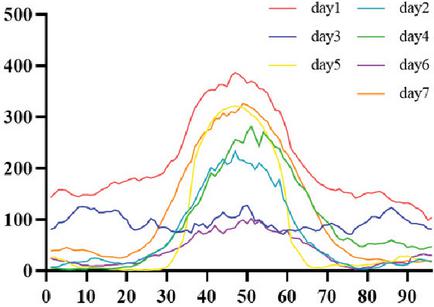
Figure 3 Binary method for clustering typical days.
Although the dynamic reserve capacity curve offers significant innovation, its practical implementation faces challenges such as high-frequency data acquisition and regulatory acceptance. However, modern SCADA and EMS systems in China already provide the necessary data infrastructure. For regulatory integration, a “dual-track” approach is recommended, where the dynamic curve initially serves as a benchmark for traditional fixed-margin requirements before transitioning to a full settlement role as the market matures.
3.3 Performance Payment Based on the Dynamic Reserve Capacity Demand Curve
As an integral part of the capacity market, the judgment criterion for the scarcity condition of performance payment is usually the adequacy of the system’s available capacity. However, a fixed capacity demand criterion cannot well reflect the changes in capacity demand under different energy scenarios and is low in economic efficiency. For this reason, based on the dynamic capacity demand curve proposed in the previous section, this section takes into account the seasonal output differences and flexible adjustable characteristics of different types of generating units to reflect the inherent value of capacity more accurately, and takes the real-time flexible dispatching capacity of units as the criterion for scarcity judgment in combination.
Seasonal characteristics have been reflected in the dynamic reserve capacity curve, and the real-time dispatching of reserve capacity is mainly undertaken by hydropower and thermal power units. The real-time dispatchable resources, together with the peak regulation depth, ramping rate of units and the reliability requirement criteria of the power system, are shown in Table 2.
Table 2 Adjustable unit parameters
| Category | Index | Specification |
| Thermal Power | Peak Regulation Depth | 40%50%, over 50% for some units |
| Ramping Rate | 1%2% per minute, 3%6% per minute for some units | |
| Hydropower | Peak Regulation Depth | / |
| Ramping Rate | 50%100% per minute | |
| Reliability | – | Deviation of 0.2 Hz: no more than 30 minutes |
| Standard | Deviation of 1 Hz: no more than 15 minutes |
Therefore, the scarcity judgment criterion for reserve capacity, which is calculated based on the peak regulation depth and ramping rate of units as well as the reliability requirements of the power system, is given as follows:
| (20) | |
| (21) |
Wherein, denotes the dynamic reserve capacity requirement at time t, and represents the real-time flexible adjustable capacity of the system at time t. A capacity scarcity event is formally triggered when the dynamic reserve requirement exceeds the available flexible capacity. For the individual unit constraints in Equation (21), v is the ramping rate of the unit, is the response time requirement dictated by system reliability standards (e.g., 15 or 30 minutes), D represents the peak regulation depth, is the installed capacity of the unit, and denotes the real-time available capacity margin of the unit. The flexible capacity is dynamically constrained by the unit’s ramping capability, peak regulation depth, and actual available margin.
4 Case Study
4.1 Case Setup
In this paper, a case calculation is carried out based on the historical actual wind and photovoltaic power generation data of Yunnan Province and the runoff data in 2022. Meanwhile, the power generation and daily load are scaled in consideration of the actual installed capacity ratio of different energy types (wind, photovoltaic, hydropower, thermal power) in the province. After scaling, the photovoltaic installed capacity is 400 MW, the wind installed capacity is 300 MW, the thermal power unit capacity is 1000 MW, and the hydropower unit capacity is 1618 MW. To reflect the seasonal characteristics of wind, photovoltaic and hydropower generation more accurately, the months are reordered for greater clarity, as shown in Table 1. Seven typical days in each distinct wind-hydrological period are selected for calculation in this paper to evaluate the effects of the monthly capacity auction and the new reserve capacity compensation mechanism. Table 1 shows the wind and hydropower generation in each month. According to the variations in hydropower and wind power, a year can be roughly divided into five time periods. However, since photovoltaic power generation is less affected by seasonal factors, no separate classification is conducted for it.
4.2 Calculation of Hydropower Generation
The hydropower generation in this paper is calculated based on a method for power generation calculation using the effective runoff per ten-day period [21]. The output fluctuations of hydropower units within each ten-day period are neglected, and the power generation is calculated on a ten-day basis. As most hydropower stations in Yunnan Province are run-of-river type with small reservoir capacity and low water storage capacity, the inflow balance operation mode is adopted for all reservoirs in this calculation, with a water head of 65 meters. Setting the hydraulic head at a constant 65 meters is a practical approach for this analysis. In Yunnan Province, most hydropower facilities operate as run-of-river plants with very little storage. Consequently, their upstream water levels barely fluctuate during daily dispatch. When looking at historical records from typical plants in the area, the daily head variation rarely exceeds 2% or 3%. For the macro-level capacity and generation estimates conducted in this study, a fluctuation this small doesn’t meaningfully alter the mathematical Capacity Balance Constraintresults. Ultimately, holding the head constant cuts down on computational demands without sacrificing the required precision. Based on the historical data of the power station at a water head of 65 meters under different inflow rates, the inflow rate range during the period of maximum power generation is [Qm, Qn]. The inflow rate Q is divided into two intervals: QQn and QQm, and the relationship between the inflow rate Q and power generation E is plotted via a linear regression equation.
Figure 4 shows the linear regression equations and curves for QQn and QQm.
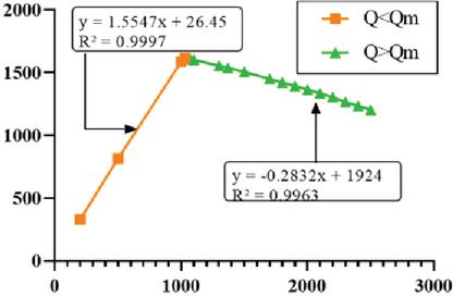
Figure 4 Reserve capacity for hydropower.
4.3 Calculation of the Reserve Capacity Demand Curve
In this paper, the error probability models reflecting the characteristic differences of geographical and climatic conditions in different periods and seasons are fitted via the non-parametric kernel density estimation method based on historical data. Since only the issue of capacity upward adjustment is discussed in this paper, the parts of wind and photovoltaic power data where the actual output exceeds the predicted value are excluded, and the modeling is only conducted for the parts where the actual power generation is lower than the predicted value. Meanwhile, to simplify the model and integrate the output uncertainties of wind and photovoltaic power, a holistic modeling is performed for the two types of units. Figure 5 shows the error probabilities in different periods.
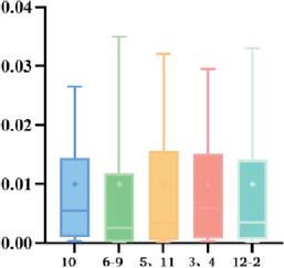
Figure 5 Error probability.
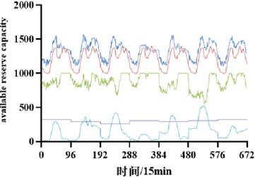
Figure 6 Load and standby for December, January and February.
Assuming a confidence probability of 99.9% – i.e., the output error of wind and photovoltaic power is lower than the reserve capacity reserve in 99.9% of cases – the results for the 12 months can be calculated and are presented as a bar chart in Figure 6. Given the model scaling in this simulation, the actual installed capacity of wind power in Yunnan Province is 8.9139 GW and that of solar power is 4.4003 GW, with the maximum installed capacity of a single unit in the system set at 1000 MW. Based on the model scaling ratio, the system’s contingency reserve is calculated as 52.5754 MW (corresponding to the maximum unit capacity), and the net load reserve is set at 5% of the scaled maximum daily load for working days in the province (the actual working day maximum load is approximately 18500 MW), resulting in a value of 48.6322 MW.
4.4 Clustering and Simulation
Based on the output characteristics of wind and photovoltaic power data in each time period, the data are clustered into seven typical days, and simulations are conducted on the capacity performance of these typical days in each period, with details shown in Figures 6–7. The black curve represents the capacity and reserve required by the power system, and the colored bar charts represent the current power generation capacity and available reserve capacity of various types of generating units. The blank areas formed where the total height of the bar charts is lower than the black curve indicate the occurrence of capacity scarcity. Since the clustering is conducted on a daily basis, significant differences exist among the daily data within a week’s dataset.
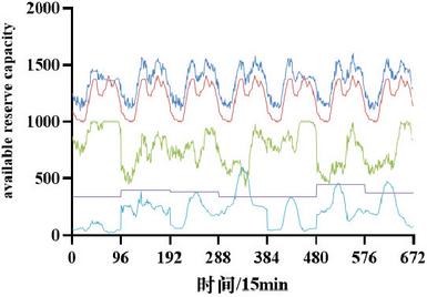
Figure 7 Load and standby for March and April.
Finally, simulation experiments are conducted for the five time periods with distinct wind and photovoltaic conditions based on the dynamic reserve capacity demand, so as to verify the compensation and incentive effects of the dynamic payment mechanism and its performance payment on flexible capacity during scarcity periods. Given the current priority dispatching of wind and photovoltaic power, their confidence capacity is taken as the capacity obligation in this paper to calculate the available flexible capacity, while no performance payment compensation is applied to wind and photovoltaic capacity.
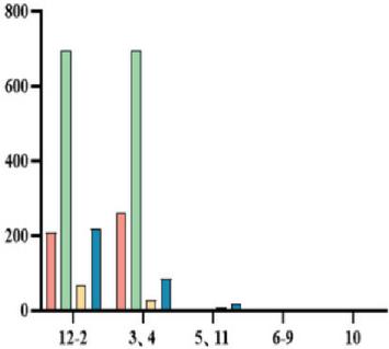
Figure 8 Performance revenue.
4.5 Result Analysis
The result analysis shows that from December to the following April, during the dry season combined with the light and moderate wind periods, hydropower and wind power have almost no surplus regulating capacity, and the real-time regulation obligation is borne almost entirely by thermal power. In some cases, the total reserve capacity is even insufficient, resulting in an extremely tight reserve capacity situation. In this period, there are not only revenues from the capacity auction market, but also performance payments triggered to provide incremental compensation for the available capacity during scarcity periods. In May and November (the normal water period), hydropower generation remains limited. Although the output of wind and photovoltaic power is relatively high in the strong wind period, the regulating capacity of hydropower can meet most of the regulation requirements, leading to a low demand for thermal power.
The capacity auction price in the auction market is zero, despite the performance payments triggered by certain fluctuations. From June to September (the light wind period), the output of wind and photovoltaic power is low, yet the output of hydropower in the wet season is far higher than the reserve demand. Thermal power units are barely required to participate in additional regulation, and hydropower units can meet the demand for the full load and regulating capacity for the most part, resulting in sufficient reserve capacity. In October, under the combined conditions of the strong wind period and wet season, the output of new energy is robust, and the regulating capacity of hydropower remains highly abundant with sufficient reserve capacity in the system.
5 Conclusions
Through a comparative analysis of the market design for performance payment and capacity auction, three conclusions are drawn as follows:
The available power generation during peak periods may be lower than the reserve capacity required by the power system, which triggers performance payments and helps alleviate the revenue gap of flexible adjustable units.
Compared with capacity auction, performance payment features a more timely price signal and higher price elasticity.
The amount of performance payment is correlated with the PPR (Performance Payment Rate), and it is difficult to determine an appropriate value in the initial stage of the market.
References
[1] Cramton P, Stoft S. A Capacity Market that Makes Sense[J]. Papers of Peter Cramton, 2005, 18(7): 43–54.
[2] Zhang Juntao, Cheng Chuntian, Yu Shen, et al. Progress, Challenges and Prospects of Research on Hydropower Supporting the Flexibility of New Power System[J/OL]. Proceedings of the CSEE: 1-22 [2024-03-28].
[3] Liu Juan, Zhang Xiuzhao, Wang Zhimin, et al. Problems in Yunnan Electric Power Development and Suggestions for the Future Development of New Electric Power System[J]. Yunnan Electric Power, 2021, 49(04): 2–5.
[4] Agah M M. Operating Reserve Requirement of Power Systems with High Penetration of Wind Power[J]. IEEE Transactions on Power Systems, 2015.
[5] Meng Yiqun, Cao Yuwei, Li Jinqiu, et al. The Real Cost of Deep Peak Shaving for Renewable Energy Accommodation in Coal-Fired Power Plants: Calculation Framework and Case Study in China[J]. Journal of Cleaner Production, 2022, 367.
[6] Tan H, Li M, Ma T, et al. Research on the Participation of Load-Side Resources in Auxiliary Services under the Background of New Power System[C]. 2022 6th International Conference on Power and Energy Engineering (ICPEE), Shanghai, China, 2022.
[7] National Development and Reform Commission of the People’s Republic of China. Notice of the National Development and Reform Commission and the National Energy Administration on Establishing a Capacity Tariff Mechanism for Coal-Fired Power [EB/OL].
[8] Batlle C, Vázquez C, Rivier M, et al. Enhancing Power Supply Adequacy in Spain: Migrating from Capacity Payments to Reliability Options[J]. Energy Policy, 2007, 35(9): 4545–4554. DOI:10.1016/j.enpol.2007.04.002.
[9] T Georgios, P Konstantinos, M Prodromos, et al. A Shortage Pricing Mechanism for Capacity Remuneration with Simulation for the Greek Electricity Balancing Market[J]. Utilities Policy, 2021, 71.
[10] Hasani-Marzooni M, Hosseini H S. Dynamic Analysis of Various Investment Incentives and Regional Capacity Assignment in Iranian Electricity Market[J]. Energy Policy, 2013, 56: 271–284.
[11] Hogan M. Follow the Missing Money: Ensuring Reliability at Least Cost to Consumers in the Transition to a Low-Carbon Power System[J]. The Electricity Journal, 2016, 30(1): 55–61.
[12] Krapels E, Flemming P, Conant S. The Design and Effectiveness of Electricity Capacity Market Rules in the Northeast and California[J]. The Electricity Journal, 2004, 17(8): 27–32.
[13] Wang Dongming, Li Daoqiang. Analysis of the PJM Electricity Capacity Market in the United States[J]. Zhejiang Electric Power, 2010, 29(10): 50–53.
[14] Chen Xi, Zang Xiaofei, Song Yang. Analysis of the UK Electricity Capacity Market and Its Enlightenments[J]. Power System Engineering, 2019, 35(02): 80–82.
[15] Liang Jiahao, Liu Dunnan, Shi Lianjun, et al. Design of Medium- and Long-Term Reserve Capacity Market Mechanism Accommodating the Participation of Emerging Entities[J/OL]. Power System Technology: 1-16 [2026-03-22].
[16] Khoshjahan M, Fotuhi-Firuzabad M, Moeini-Aghtaie M, et al. Enhancing Electricity Market Flexibility by Deploying Ancillary Services for Flexible Ramping Product Procurement[J]. Electric Power Systems Research, 2021, 191: 106878.
[17] Liang Y, Guo C, Ding Z, et al. Agent-Based Modeling in Electricity Market Using Deep Deterministic Policy Gradient Algorithm[J]. IEEE Transactions on Power Systems, 2020, 35(6): 4180–4192.
[18] Cramton P, Stoft S. A Capacity Market that Makes Sense[J]. Papers of Peter Cramton, 2005, 18(7): 43–54.
[19] PJM Interconnection. PJM Manual 18: PJM Capacity Market [R/OL]. Audubon, PA: PJM Interconnection LLC, 2022. Available at: https://www.pjm.com/library/manuals.
[20] National Energy Administration of the PRC. Technical guide for configuration of accident reserve capacity in power systems: DL/T 2238-2021 [S]. Beijing: China Electric Power Press, 2021.
[21] Liu Zhiwu. A method for rapid calculation of hydropower station generation capacity: China, CN105096216A [P]. 2015-11-25.
Biographies

Wei Guangxu, Male, postgraduate student at the School of Electrical Engineering, Northeast Electric Power University, majoring in Electrical Engineering. His main research interests include electricity market, capacity market, and optimal power dispatch.

Dong Shuo, Male, postgraduate student at the School of Electrical Engineering, Northeast Electric Power University, majoring in Electrical Engineering. His main research interests include electricity market, capacity market, and optimal power dispatch.
Strategic Planning for Energy and the Environment, Vol. 45_3, 791–812
doi: 10.13052/spee1048-5236.4537
© 2026 River Publishers