Distributed Photovoltaic Hosting Capacity Evaluation for Distribution Networks Considering Medium-Voltage and Low-Voltage Interactions
Yinghua Sun1,*, Chuang Liu1, Ruifeng Li1, Dongbo Guo2 and Fengyue Zhao1
1School of Electrical Engineering, Northeast Electric Power University, Jilin, Jilin, 132012, China
2Tsinghua University, Beijing, 100084, China
E-mail: 2081202160@qq.com
∗Corresponding Author
Received 12 March 2026; Accepted 21 April 2026
Abstract
Under the “Dual Carbon” goals background, large-scale integration of distributed photovoltaics (PV) is transforming distribution networks from passive radial systems into active bidirectional interactive systems. To address this, this paper proposes a hosting capacity assessment method for high-penetration distributed PV in distribution networks that considers medium and low voltage levels (MV-LV) interactions. First, by analyzing the impacts of MV-LV grid interactions, four core interaction mechanisms are identified: considering voltage coupling under low-voltage saturation, current coupling under short-circuit superposition, and power coupling under photovoltaic concentration. An MV-LV interaction model is constructed based on these mechanisms. Subsequently, the concept of a Voltage Deviation Index (VDI) is introduced to quantify the voltage quality level of the system. An assessment model is then formulated with the dual objectives of maximizing PV hosting capacity and minimizing VDI, incorporating system-wide constraints, MV-specific and LV-specific constraints, as well as MV-LV interaction constraints. Finally, a Differential Evolution Non-dominated Sorting Whale Optimization Algorithm (DE-NSWOA) is employed to solve. The effectiveness of the proposed method is validated through simulations based on a 10 kV distribution network in a city in East China, providing a foundation for subsequent research.
Keywords: MV-LV interaction in distribution networks, distributed photovoltaics, hosting capacity, improved differential evolution non-dominated sorting whale optimization algorithm.
1 Introduction
As a clean energy source, PV systems have been widely integrated into medium and low voltage distribution networks [1]. The rapid development of distributed PV has transformed distribution grids from traditional “passive” unidirectional radial networks into “active” bidirectional interactive systems, making bidirectional power flow the new normal [2, 3]. However, due to the stochastic and intermittent nature of PV generation [4–6], large-scale integration may lead to issues such as voltage violations and uneven power flow distribution [7, 8].
China’s National Energy Administration explicitly requires “assessing distribution network hosting capacity and establishing a release and early warning mechanism for renewable energy integration potential” [9]. This marks a new phase of refined, dynamic, and intelligent hosting capacity assessment for distribution networks in China. Traditional hosting capacity evaluation primarily focused on static capacity limits, determined by critical equipment ratings, with insufficient consideration of load and PV dynamics [10–13].
The PV hosting capacity refers to the maximum PV capacity that can be accommodated while ensuring safe operation, power quality, and equipment limits [14–16], specifically defined as the maximum active power output of distributed PV systems under standard test conditions. Currently, distribution networks in central and eastern China are nearing saturation, with increasing warnings of insufficient hosting capacity. Some regions have even suspended new distributed PV project approvals [17], highlighting the urgency and necessity of improving hosting capacity assessment methods.
Current hosting capacity assessment methods mainly include deterministic power flow analysis [18], probabilistic methods [19], and optimization algorithms [20–23]. Probabilistic methods treat PV output and load as random variables, simulating various operating scenarios through extensive random sampling to statistically determine the probability of voltage violations or equipment overloads. However, these methods face challenges such as computational complexity and high dependence on data accuracy. Optimization-based methods can achieve theoretical optimal solutions and simultaneously optimize devices such as on-load tap changers and reactive power compensation equipment, further enhancing hosting capacity.
Several studies have addressed the problem of distributed PV hosting capacity assessment. Reference [19] introduced “probabilistic hosting capacity,” establishing normal probability density functions for each uncertain parameter and using statistical simulations to evaluate hosting capacity. While the results were significantly higher than deterministic assessments, the model was relatively complex. Reference [20] developed a hosting capacity model targeting maximum wind and PV integration capacity, solved via second-order cone programming. However, it did not resolve the subjectivity of weight assignment. Reference [21] considered both PV output volatility and load uncertainty, employing Monte Carlo simulation for multi-scenario input generation and Latin hypercube sampling to improve efficiency, albeit with high computational cost. Reference [22] improved network analysis and entropy weight methods for comprehensive weighting, building a multi-dimensional index system covering safety, economy, and structural stability, combined with TOPSIS for dynamic node criticality ranking to prioritize high-risk nodes. Reference [23] proposed a sequential Monte Carlo simulation-based reliability assessment.
In summary, traditional PV hosting capacity assessment methods often focus on a single voltage level, neglecting interactions between whole distribution networks. Moreover, most designs prioritize maximizing renewable energy hosting capacity, with insufficient attention to voltage quality, leading to power quality degradation as PV integration increases.
To address these challenges, this paper proposes a hosting capacity assessment method for high-penetration distributed PV in distribution networks, considering MV-LV interactions. First, the impacts of MV-LV grid interactions are analyzed, and four core interaction mechanisms are proposed: cross-level voltage propagation, hybrid short-circuit current superposition, harmonic resonance path expansion, and reverse power transient impacts. A system model incorporating MV-LV interactions is then constructed based on these mechanisms. Next, system voltage quality is quantified, with dual objectives of maximizing PV hosting capacity and optimizing voltage quality. An IDE-NSWOA is proposed to solve the model.
2 MV-LV Distribution Network Interaction Model
With the continuous increase in distributed PV penetration, the energy interaction between MV and LV distribution networks has shifted from the traditional unidirectional power supply mode to a complex multi-directional coupled mode [24]. Driven by this transformation, emerging interaction effects such as superimposed voltage fluctuations and hybrid short-circuit currents have become increasingly prominent. Conventional methods that analyze MV and LV networks in isolation are gradually proving inadequate for accurately assessing system hosting capacity.
Building upon existing models for power flow, voltage, and other aspects of MV-LV distribution networks, this section develops interaction models for voltage, current, power, and frequency by incorporating MV-LV coupling relationships. Furthermore, four core interaction mechanisms between MV and LV networks are proposed, establishing a theoretical foundation for the holistic assessment of the distribution system presented in subsequent sections.
2.1 Distribution Network Power Flow Model
The MV distribution network employs a symmetrical positive sequence model, with the node voltage and power balance relationship described as follows:
| (1) |
among them: and are the active and reactive power of the node ; is the voltage of node ; is the element of the node admittance matrix.
In low-voltage distribution networks, considering three-phase unbalance, a three-phase power flow model is adopted. For phase at node :
| (2) |
Where, and are the active and reactive power of phase at node , respectively; is the voltage of phase at node ; is the mutual admittance between phase of node and phase of node in the nodal admittance matrix. In a three-phase system, each element of the nodal admittance matrix is no longer a single complex number but a 3 3 matrix:
| (3) |
Considering data availability and computational complexity, the simplified low-voltage distribution network model is as follows:
| (4) |
2.2 Impact of MV-LV Interaction on Distribution Networks
The coupling effect between distributed photovoltaics in medium- and low-voltage distribution networks is a key link in hosting capacity assessment, which results in strong coupling between medium- and low-voltage distribution networks in terms of voltage, current and power. Traditional assessment methods often split the medium- and low-voltage networks for analysis, ignoring the dynamic connection between them. This section focuses on discussing the impact of coupling in these three aspects and proposes corresponding quantitative assessment methods.
(1) Voltage Coupling Considering Low-Voltage Saturation
The coupling effect of voltage fluctuations between the medium-voltage and low-voltage sides of the distribution network cannot be ignored. Voltage fluctuations on the medium-voltage side can be transmitted to the low-voltage side through the transformer, and vice versa. The impact of medium-voltage voltage fluctuations on the low-voltage side is:
| (5) |
where is the voltage fluctuation on the low-voltage side; is the voltage fluctuation on the medium-voltage side.
Based on the fluctuation relationship between the two sides, the overall expression of voltage coupling on the medium- and low-voltage sides is obtained:
| (6) |
where is the equivalent admittance on the low-voltage side.
When the access of distributed PV exceeding the limit on the low-voltage side causes the voltage rise to reach saturation, it leads to an increase in the voltage of the low-voltage bus, which is transmitted to the medium-voltage side through the distribution transformer. This cross-level transmission effect may cause an overall increase in the voltage of the medium-voltage feeder. For this reason, the Voltage Penetration Coefficient (VPC) is introduced to characterize the change in the voltage of the transformer district node for every 1 kW increase in the grid-connected capacity of low- voltage PV.
| (7) |
where represents the percentage change in MV bus voltage, and represents the total power variation of LV photovoltaic generation. The voltage deviation in MV grids is generally required to be controlled within 5% to 10% of the nominal voltage. If the VPC ratio is 0.5%/MW, it implies that a 10 MW increase in PV capacity could lead to a voltage change of up to 5%, which is already approaching the allowable limit. Intervention is necessary to prevent exceeding the boundary. When the VPC exceeds 0.5%/MW, it indicates that the local absorption capacity of PV on the LV side is nearing saturation, which can easily impact the voltage stability of the MV side, requiring measures for voltage regulation.
(2) Current Coupling Considering Short-Circuit Superposition
The coupling effect between medium- and low-voltage distribution networks is particularly prominent at the fault current level. When a short-circuit fault occurs in the distribution system, distributed photovoltaics on the low-voltage side can inject short-circuit current into the fault point through grid-connected inverters, which superimposes with the fault current on the medium-voltage side. This superposition effect will change the operating characteristics of the original relay protection system, thereby causing problems such as misoperation or refusal to operate of protection devices.
For ease of analysis, the total short-circuit current at the short-circuit fault point can be decomposed into two components, with the mathematical expression as follows:
| (8) | |
| (9) |
where is the total short-circuit current on the MV side; is the short-circuit current contribution from the MV side excluding that from PV systems; is the equivalent short-circuit current contributed by the i-th low-voltage PV inverter to the MV side, typically calculated as 1.1 to 1.5 times its rated current; is a coefficient; and is the rated short-circuit current of the i-th PV inverter.
| (10) |
where represents the short-circuit current contributed by the i-th LV PV system to the MV side after conversion, typically calculated as 1.11.5 times the rated current of the inverter; while denotes the short-circuit current on the MV side excluding the PV contributions. Since the interrupting capacity of medium-voltage circuit breakers is typically designed to be 100%–120% of the rated short-circuit current, if the SCR exceeds 5%, it indicates that the short-circuit capacity contributed by PV systems accounts for a significant proportion of the total medium-voltage short-circuit capacity. This may trigger overcurrent protection in the inverters themselves and affect protection criteria under asymmetric short-circuit conditions due to current superposition. The total short-circuit current may approach or exceed the rated value of the circuit breaker, leading to interruption failure or equipment damage, necessitating recalibration of protection settings.
(3) Power Coupling Considering Photovoltaic Concentration
The dynamic characteristics of the coupling between distributed photovoltaics in medium- and low-voltage networks are also reflected in the impact of PV output fluctuations and load fluctuations on the medium-voltage network transmitted through low-voltage transformers. The power transmission relationship of the transformer is:
The total fault current at the short-circuit point is the sum of the short-circuit current from the MV system and the current contributed by the LV photovoltaic systems, expressed as:
| (11) | |
| (12) |
where is the total short-circuit current on the MV side; is the short-circuit current contribution from the MV side excluding that from PV systems; is the equivalent short-circuit current contributed by the i-th low-voltage PV inverter to the MV side, typically calculated as 1.1 to 1.5 times its rated current; is a coefficient; and is the rated short-circuit current of the i-th PV inverter.
When LV photovoltaics generate concentrated power, it may cause reverse power to flow back to the MV side through transformers, leading to congestion in MV lines or misoperation of protection devices. We introduce the Reverse Congestion Index (RCI) to represent the ratio of peak reverse power to the thermal stability capacity of MV lines:
| (13) |
where represents the peak reverse power flow on the MV line, and denotes the line’s thermal stability capacity. Line overload protection settings are typically set at 90%–110% of the thermal stability capacity. Considering safety margins and economic optimization, setting the RCI limit at 0.8 ensures sufficient time to initiate flexible control measures such as PV power curtailment or energy storage regulation before protection activation.
3 Scene Reduction Considering Source-Load Uncertainty
The output of distributed photovoltaics (PV) and the load fluctuation in distribution networks exhibit significant randomness and uncertainty. Improper selection of evaluation scenarios may lead to overly optimistic or conservative assessment results. The multi-scenario analysis method can effectively reduce the complexity of problem solving while ensuring the solution accuracy of the optimal configuration scheme, transforming a large number of uncertain scenarios into a small number of representative deterministic scenarios, thereby improving the evaluation accuracy.
The scenario clustering method based on historical data performs clustering division by calculating the spatial distance between scenarios, and classifies scenarios with high similarity into the same category, thus realizing the reduction of the scenario set. This method can avoid the huge computational burden of the Monte Carlo method and the subjectivity of fuzzy optimization, and remains effective when the number of original scenarios is large. Therefore, this paper adopts cluster analysis to carry out the research on generating typical scenarios.
The K-means algorithm has certain application limitations when dealing with scenarios with complex and variable PV output fluctuations and load characteristics in distribution networks. The optimized K-means++ algorithm, based on K-means, adopts the farthest point priority selection mechanism based on probability weight to improve the generation process of initial cluster centers, effectively alleviating the problem that the traditional K-means algorithm is highly sensitive to initial cluster centers, greatly enhancing the stability of clustering results, and improving the overall convergence efficiency of the algorithm.
Compared with hierarchical clustering methods, K-means has higher computational efficiency, which is especially suitable for processing large-scale datasets and can quickly meet the analysis requirements of massive operation data in distribution networks. Meanwhile, compared with density-based clustering methods, K-means does not need to pre-set density-related thresholds, and can better adapt to the non-uniform distribution characteristics of distributed PV output and load demand in distribution networks.
The implementation steps of K-means are as follows:
(1) This paper adopts the elbow method to determine the optimal number of clusters. This method takes the sum of squared errors (SSE) as the core evaluation index, whose physical meaning is the sum of the squared Euclidean distances from each sample point to the corresponding cluster center. As the number of clusters K increases gradually, the SSE shows an overall monotonic downward trend; when K is less than the real number of clusters, the SSE decreases significantly; when K reaches the actual number of clusters, further increasing the number of clusters has a significantly weakened effect on improving the SSE, and the curve slope changes sharply to form an “elbow” inflection point. The K value corresponding to the inflection point of the curve is the optimal number of clusters.
(2) Initialization. Randomly select one sample from the data sample set as the first initial cluster center.
(3) Calculate the Euclidean distance between each sample point and the currently determined cluster centers one by one.
(4) Construct a probability selection model based on the Euclidean distance from each data point to the existing cluster centers, so that sample points farther from the existing centers have a higher probability of being selected as the next cluster center.
(5) Repeat steps (2) to (4) until all K initial cluster centers are selected.
4 Evaluation Model
The core MV-LV interaction mechanisms proposed in the previous sections expand the evaluation dimensions of distribution network hosting capacity and address the shortcomings of traditional methods in considering voltage coupling, quantitative short-circuit contribution, and resonance risk identification. Based on these mechanisms, this chapter constructs a distributed PV hosting capacity assessment model that incorporates MV-LV interactions.
4.1 System Voltage Quality Assessment
The increase in PV penetration alters the power flow direction in distribution networks, leading to issues such as voltage violations and line overloads. Focusing solely on maximizing hosting capacity may mask the risk of power quality degradation. The main indicators for assessing system power quality are frequency and voltage quality. Frequency quality metrics include frequency deviation tolerance, while voltage quality metrics encompass allowable voltage deviation, waveform distortion rate (harmonics), three-phase voltage unbalance tolerance, and voltage fluctuation and flicker tolerance. For distribution networks, voltage quality is a decisive factor for power supply reliability.
In addition to evaluating maximum PV hosting capacity, this paper introduces a Voltage Deviation Index (VDI) to quantify the extent of deviation of various voltage quality indicators from standard values. VDI indicates poorer voltage quality. The VDI is calculated using the entropy weight method, with the steps as follows:
(1) Select indicators reflecting system voltage quality. This paper selects four indicators to assess voltage quality: voltage deviation , total harmonic distortion rate , three-phase voltage unbalance and voltage flicker .
(2) Formation of voltage quality data matrix. A network voltage quality data matrix is created using the voltage quality indicators. The data is normalized using the min-max standardization method to eliminate dimensional effects. The formula for normalization is as follows:
| (14) |
(3) Calculation of entropy values for each indicator. The entropy value for each indicator is calculated using the following formula:
| (15) |
where is the entropy value of the -th indicator; is the proportion of the normalized value of the -th indicator in the -th dataset; is a constant; is the number of datasets.
(4) Calculation of weights for each indicator. The weights for each indicator are calculated using the formula:
| (16) |
where is the weight of the -th indicator; is the total number of indicators.
(5) Derivation of system VDI from indicator weights. The system VDI is calculated using the following formula:
| (17) |
where is the time; is the normalized value of the v-th voltage quality indicator at time , with the reference value being the national standard for the maximum allowable short-term deviation for each indicator.
The implementation methodology for measuring the system voltage quality based on VDI is illustrated in Figure 1. Simulation verification shows that, considering long-term non-violation and safety margins, the system VDI should generally not exceed 0.75.
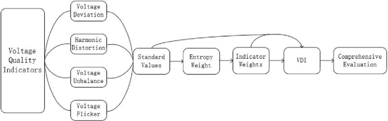
Figure 1 System voltage quality assessment.
4.2 Objective Function
(1) Maximum installed capacity of distributed PV
| (18) |
(2) Minimum VDI
| (19) | |
| (20) |
in the equation, represents the Voltage Deviation Index on the MV side; denotes the total number of LV distribution units; indicates the Voltage Deviation Index of the num-th LV distribution unit.
4.3 Constraints
(1) The overall constraints of the power distribution system
Power flow constraints:
| (21) |
In the equation: represent the active and reactive power output of the distributed photovoltaic system connected at node denote the active and reactive power load at node are the conductance and susceptance elements of the nodal admittance matrix.
Voltage deviation constraints:
| (22) |
in the formula: represents the node voltage; denotes the nominal system voltage; is the permissible voltage deviation limit. However, due to the smaller base value, the actual allowable absolute deviation is smaller, requiring higher accuracy in assessments.
Thermal stability constraints:
| (23) |
where represents the current on branch ; denotes the maximum allowable current for branch .
PV inverter capacity limitations:
| (24) |
in the equation: represents the rated apparent power of the inverter; denotes the active power output from the PV inverter; is the reactive power provided by the inverter.
(2) Unique constraints on medium and low voltage sides
The MV distribution network has a wide supply range and a large load capacity, typically equipped with various reactive power regulation devices. The MV side has high requirements for voltage stability and power quality, necessitating management of reactive power across the entire region to ensure that voltage levels remain within target ranges, thereby avoiding impacts on the operation of downstream LV distribution networks.
The expression for reactive power regulation constraints on the MV side is as follows:
| (25) |
The LV distribution network directly supplies power to residential, commercial, and small industrial users. Its single-phase loads are significant, with low tolerance for voltage fluctuations and high randomness in usage behavior, which can easily cause three-phase imbalance. The neutral line directly connects to users, and during three-phase imbalance, it may carry large currents, leading to neutral line overload and even fire hazards. In contrast, the loads on the MV distribution network are aggregated through transformers, which typically mitigates the issue of three-phase imbalance. The neutral point of the MV network is usually grounded through an arc suppression coil or resistor, meaning that unbalanced current does not pass through the neutral line, posing less risk. Therefore, the LV distribution network must pay special attention to the issue of three-phase imbalance.
Based on the calculation method for voltage imbalance defined by IEEE Std 112–1991, constraints are applied to the Phase Voltage Unbalance Rate (PVUR) as follows:
| (26) |
where represents the permissible maximum phase voltage unbalance rate. The PVUR is calculated as follows:
| (27) | |
| (28) |
where, , , represent the root-mean-square (RMS) values of phase A, B, and C voltages.
(3) Interaction constraints between medium and low voltage
Constraints are applied to the four core interaction mechanisms proposed in the previous sections:
| (29) | |
| (30) | |
| (31) | |
| (32) |
where represents the maximum allowable voltage penetration coefficient; denotes the maximum permissible short-circuit contribution ratio; is the low-risk minimum frequency point; indicates the maximum allowable reverse congestion rate. The evaluation incorporates real-time adjustments through system reactive power compensation:
| (33) |
where, represents the dynamic reverse load ratio threshold; denotes the equipment rated apparent power.
Transformer capacity constraints:
| (34) |
where represents the transformer’s operational apparent power; denotes the transformer’s maximum rated capacity.
4.4 Improved DE-NSWOA Model
Based on the NSWOA model, this paper proposes an improved DE-NSWOA solution model. NSWOA is a multi-objective optimization algorithm that integrates Pareto dominance relations and the Whale Optimization Algorithm (WOA). Its core idea combines the multi-objective processing framework of NSGA-II with the search mechanism of WOA, incorporating Pareto dominance and crowding distance to identify the optimal solution set.
First, to address the issue that the three search modes of WOA – random search, spiral updating, and shrinking encircling – exhibit a progressively hierarchical relationship and are significantly influenced by random factors in traditional search mechanisms, this paper proposes a novel individual search mechanism for NSWOA.
An Update Distance (UPD) is defined to quantitatively describe the degree of optimization in an individual’s position before and after an iteration. The formula is as follows:
| (35) |
where represents the current generation, and denotes the value of the objective function at generation . The proposed search mechanism is jointly determined by the iteration stage and UPD, aiming to better balance global and local exploration, thereby forming the improved NSWOA. The specific implementation of the individual search mechanism is expressed as follows:
| (36) |
where is the expected number of iterations for NSWOA convergence, and is the set threshold for the update distance.
However, challenges such as susceptibility to local Pareto optimal fronts and sensitivity to parameters persist. To address these issues, this paper integrates the mutation-crossover mechanism of Differential Evolution (DE) with the improved NSWOA, resulting in the improved DE-NSWOA algorithm. The introduction of DE aims to enhance the global search capability and solution set diversity of NSWOA in multi-objective problems, preventing premature convergence to local Pareto optimal fronts. Specifically, after updating the Pareto archive in each iteration of NSWOA, DE operations are performed on a subset of individuals. The implementation process of incorporating DE is as follows:
(1) Target individual selection. Individuals not in the first front are selected to undergo the DE operation, while elite solutions in the first front are preserved to avoid disrupting high-quality solutions.
(2) Differential mutation. For each target individual three distinct individuals , and are randomly selected to generate a mutation vector :
| (37) |
where is the scaling factor that controls the differential step size;
(3) Binomial crossover. The mutation vector undergoes crossover with the original individual Xi to generate the trial vector :
| (38) |
where ;
(4) Elite selection. The trial vector and the original individual are compared based on Pareto dominance, retaining the better solution:
| (39) |
If and are non-dominated with respect to each other, the solution with a larger crowding distance (i.e., the less crowded one) is selected to maintain diversity.
By incorporating differential mutation and crossover, the population diversity is enhanced, preventing the algorithm from getting trapped in local optima. The example of differential mutation is illustrated in Figure 2, while the crossover process is demonstrated in Figure 3.
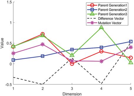
Figure 2 Example of differential mutation.
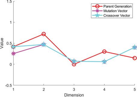
Figure 3 Example of crossover.
After the iterations are completed, the fuzzy decision-making method is used to select the optimal compromise solution from the Pareto optimal front. The procedure is as follows:
(1) Normalization of objective values. For that should be maximized (where larger values are better), the normalization formula is:
| (40) |
where is the membership degree of ; represents each outcome value in the Pareto front. For , where smaller results are preferred, its normalization formula is:
| (41) |
(2) Comprehensive membership degree calculation. A conservative strategy is adopted by taking the minimum membership degree of the two objectives:
| (42) |
(3) Optimal Solution Selection. The optimal solution is the one that minimizes the following expression.
To summarize, the implementation steps of DE-NSWOA are as follows:
Step 1: Parameter Configuration
Set the input parameters.
Step 2: Initial Population Generation
Initialize the population randomly, where each individual stores two objective function values, i.e., the individual position. Initialize the Pareto archive.
Step 3: Iteration Update
Perform one iteration for all individuals.
Step 4: Non-dominated Sorting
Step 5: Pareto Archive Update and Pruning
Update the Pareto archive by retaining only non-dominated solutions. Prune the archive by removing solutions in densely crowded regions.
Step 6: Mutation and Crossover
Perform DE mutation and crossover on individuals not in the first front using the method described earlier.
Step 7: Termination Check
Repeat Steps 3 to 6 while t=T. When t=T, output the Pareto optimal front.
Step 8: Final Solution Selection
Apply the fuzzy decision-making method to select the final solution from the Pareto optimal front.
5 Case Study Analysis
This paper takes a network of a city in East China as an example, using the distribution system shown in Figure 4 to conduct a hosting capacity assessment. Detailed load data are provided in Table 1. The topology of the MV side is shown in Figure 4(a), where the MV distribution network hosts a total distributed PV capacity of 1.74 MW, connected through eight 10/0.38 kV distribution transformers, each rated at 400 kVA. The topology of a LV transformer zone is in Figure 4(b), with PV systems integrated at nodes 32, 34, 35, and 40, each with a capacity of 18 kW. The MV feeder uses cable type YJV22-8.7 with a maximum ampacity of 450 A. The LV feeder uses cable type VV-0.6 with a maximum ampacity of 230 A.
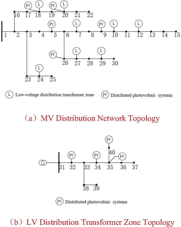
Figure 4 Medium and low voltage power distribution system.
The hosting capacity calculation requires selecting a typical time period of the year. Since distributed PV integration is most likely to cause security violations in the distribution network during summer, a typical summer day’s load and PV generation data are selected as the input, with their daily profiles shown in Figure 5. As the hosting capacity optimization problem for nodes currently without distributed PV involves siting and sizing decisions, this paper temporarily does not consider the assessment for such nodes. The three-phase load and PV data of the transformer district are listed in Table 2.
Table 1 Node load data of MV distribution network
| Node Number | Active Power Load/MW | Reactive Power Load/Mvar | Node Number | Active Power Load/MW | Reactive Power Load/Mvar |
| 1 | 0 | 0 | 16 | 0.100 | 0.046 |
| 2 | 0.115 | 0.064 | 17 | 0.095 | 0.040 |
| 3 | 0.095 | 0.038 | 18 | 0.080 | 0.033 |
| 4 | 0.050 | 0.030 | 19 | 0.080 | 0.033 |
| 5 | 0.050 | 0.020 | 20 | 0.075 | 0.030 |
| 6 | 0.195 | 0.100 | 21 | 0.060 | 0.020 |
| 7 | 0.190 | 0.100 | 22 | 0.060 | 0.018 |
| 8 | 0.070 | 0.020 | 23 | 0.180 | 0.096 |
| 9 | 0.060 | 0.015 | 24 | 0.288 | 0.155 |
| 10 | 0.060 | 0.020 | 25 | 0.100 | 0.423 |
| 11 | 0.065 | 0.022 | 26 | 0.095 | 0.044 |
| 12 | 0.065 | 0.020 | 27 | 0.086 | 0.040 |
| 13 | 0.090 | 0.043 | 28 | 0.080 | 0.038 |
| 14 | 0.055 | 0.018 | 29 | 0.080 | 0.038 |
| 15 | 0.060 | 0.020 | 30 | 0.060 | 0.033 |
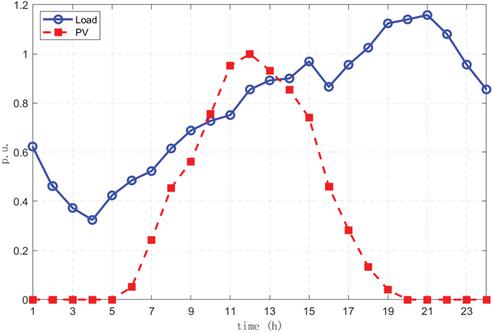
Figure 5 Typical daily load and PV generation curves.
Table 2 Three-Phase data of low-voltage transformer district
| Node | Phase A Load/kW | Phase B Load/kW | Phase C Load/kW | PV Connected Phase |
| 31 | 5.2 | 4.8 | 6.1 | – |
| 32 | 3.5 | 4.0 | 3.8 | A |
| 33 | 6.0 | 5.5 | 5.0 | – |
| 34 | 4.2 | 3.9 | 4.5 | C |
| 35 | 5.0 | 4.5 | 5.5 | C |
| 36 | 4.8 | 5.2 | 4.7 | – |
| 37 | 3.7 | 4.3 | 3.9 | – |
| 38 | 6.5 | 5.8 | 6.2 | – |
| 39 | 4.0 | 4.5 | 4.2 | – |
| 40 | 5.5 | 5.0 | 5.3 | AB |
| Total | 48.4 | 47.5 | 49.2 | – |
Table 3 MV side VDI weight calculation results
| Standardized Voltage Quality Index | ||||
| 0.20289 | 0.10688 | 1e-10 | 0.29215 | |
| 1e-10 | 0.19579 | 0.065495 | 0.033462 | |
| 0.26134 | 0.094203 | 0.12192 | 0.16165 | |
| 0.18506 | 0.10716 | 0.16207 | 1e-10 | |
| 0.17039 | 0.049052 | 0.067345 | 0.13771 | |
| 0.040849 | 0.22352 | 0.30213 | 0.066667 | |
| 0.013767 | 0.22338 | 0.10712 | 0.19434 | |
| 0.12571 | 1e-10 | 0.17391 | 0.11403 | |
| Entropy | 0.83599 | 0.88377 | 0.87371 | 0.85949 |
| Weight Coefficient | 0.29981 | 0.21247 | 0.23086 | 0.25686 |
Table 4 LV distribution transformer zone VDI weight calculation results
| Standardized Voltage Quality Index | ||||
| 1e-10 | 0.10054 | 0.14882 | 0.22178 | |
| 0.064372 | 0.12516 | 0.21483 | 0.13089 | |
| 0.16502 | 0.19566 | 0.052808 | 0.1856 | |
| 0.27367 | 1e-10 | 1e-10 | 0.16568 | |
| 0.13573 | 0.086254 | 0.13082 | 0.035658 | |
| 0.099587 | 0.29266 | 0.29381 | 0.10228 | |
| 0.1559 | 0.094389 | 0.041047 | 1e-10 | |
| 0.10571 | 0.10534 | 0.11786 | 0.15811 | |
| Entropy | 0.89284 | 0.88538 | 0.85515 | 0.89173 |
| Weight Coefficient | 0.22565 | 0.24136 | 0.30501 | 0.22798 |
Using the proposed VDI calculation method, network data sampled every two hours (i.e., 8 datasets) are used to obtain the weight results for the MV side, as shown in Table 3, and the results for an LV transformer zone are shown in Table 4. Voltage deviation has the highest weight on the MV side, whereas the three-phase voltage unbalance tolerance is the most influential indicator on the LV side. The primary reason is that MV lines are longer, making them susceptible to voltage violations at the ends due to load variations, directly affecting the power supply quality for downstream LV sides, while three-phase unbalance is generally less severe. In contrast, LV transformer zones have concentrated single-phase loads and single-phase PV integrations, leading to excessive neutral current, which can cause transformer overheating and voltage asymmetry. LV distribution networks are more prone to forming resonant circuits. Household appliances, commercial equipment, and low-power industrial devices in LV zones often use switching power supplies or power electronic devices, generating rich 3rd, 5th, and 7th harmonics. Single-phase non-linear loads causing the superposition of 3rd harmonic currents in the neutral line can easily lead to neutral overload and higher resonance risks.
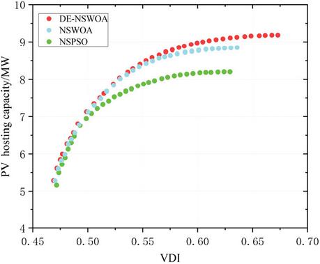
Figure 6 Pareto optimal frontier.
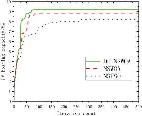
Figure 7 Convergence comparison for PV hosting capacity optimization.
The Pareto optimal solution sets generated by the improved DE-NSWOA, NSWOA, and Non-dominated Sorting Particle Swarm Algorithm (NSPSO) for optimizing hosting capacity and VDI are shown in Figure 6. The convergence comparison for the single objective of hosting capacity is shown in Figure 7. When the hosting capacity reaches a certain value, even sacrificing more VDI does not lead to a significant improvement in capacity. Among the methods, NSPSO is more prone to converging to a local Pareto front, whereas the improved DE-NSWOA demonstrates the best convergence performance. Under the same VDI, the improved DE-NSWOA achieves a higher distributed PV hosting capacity, and the DE enhancement also improves the diversity of the solutions. The final results obtained by the three methods using the fuzzy decision-making approach are presented in Table 5.
Table 5 Comparison of results using different methods
| Method | PV Hosting Capacity/MW | VDI |
| NSPSO | 7.957 | 0.561 |
| NSWOA | 8.773 | 0.601 |
| DE-NSWOA | 8.968 | 0.599 |
Using the improved DE-NSWOA and the fuzzy decision-making method, the optimal assessment results for the PV hosting capacity at MV nodes are shown in Figure 8, and the assessment results for the hosting capacity of transformer zones and their internal components on the MV side are shown in Figure 9. A comparison between the results obtained by the method proposed in this paper and those evaluated without considering medium – low voltage coupling is presented in Table 6. It can be seen that the distribution network hosting capacity considering medium – low voltage coupling is 8.968 MW, while that without consideration is 9.721 MW. Taking medium – low voltage coupling into account reduces the final hosting capacity assessment result by approximately 7.75%. The medium – low voltage coupling effect has a significant impact on the hosting capacity of medium-voltage photovoltaic systems, especially at nodes 18 and 20.
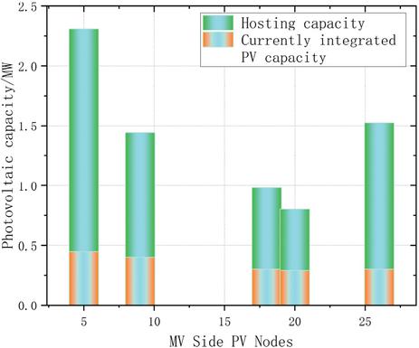
Figure 8 Assessment results of PV hosting capacity at MV-side nodes.
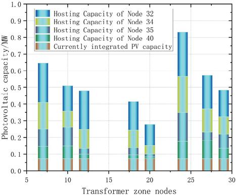
Figure 9 Assessment results of hosting capacity for MV-side transformer zones and internal components.
Table 6 Comparison between the method in this paper and the evaluation results without considering medium – low voltage coupling
| Node | Hosting Capacity Considering Medium–Low Voltage Coupling/MW | Hosting Capacity Without Considering Medium–Low Voltage Coupling/MW | |
| Medium-voltage photovoltaic | 5 | 1.861 | 1.910 |
| 9 | 1.042 | 1.150 | |
| 18 | 0.683 | 0.874 | |
| 20 | 0.515 | 0.692 | |
| 26 | 1.225 | 1.267 | |
| Distribution transformer area | 7 | 0.573 | 0.592 |
| 10 | 0.439 | 0.456 | |
| 12 | 0.408 | 0.424 | |
| 18 | 0.343 | 0.386 | |
| 20 | 0.207 | 0.243 | |
| 24 | 0.759 | 0.785 | |
| 27 | 0.501 | 0.517 | |
| 29 | 0.412 | 0.425 | |
| Total | 8.968 | 9.721 |
Table 7 Constraints limiting hosting capacity enhancement of distributed PV systems
| PV Location | Grid-connection Node | Hosting Capacity Limiting Constraints |
| MV side | 5, 20, 26 | Voltage deviation |
| 9 | Thermal stability | |
| 18 | Reactive power compensation capacity | |
| LV side | 7, 29 | VPC |
| 10 | 32, 34, 35 node: Voltage deviation 40 node: Three-phase unbalance degree | |
| 12 | 32 node: Three-phase unbalance degree 34 node: Thermal stability 35, 40 node: Voltage deviation | |
| 18 | SCR | |
| 20 | 32, 35, 40 node: Three-phase unbalance degree 34 node: Voltage deviation | |
| 24 | RCI |
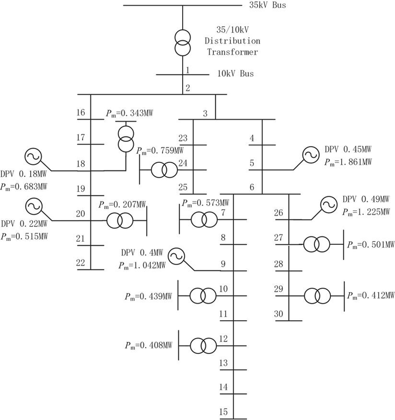
Figure 10 Evaluation results of medium and low voltage distribution network.
By analyzing the evaluation data, the primary limiting factors for enhancing the distributed PV hosting capacity can be identified. Taking the transformer zone connected to Node 20 as an example, when the hosting capacity reaches its limit, the current in the zone’s main feeder is 42.81 A, the per-unit voltage at Node 20 is 1.022, the VPC is 0.46%/MW, while the RCI reaches the threshold of 0.8. In this case, the primary solution for enhancing the hosting capacity in the zone connected to Node 20 should first address the reverse congestion issue, primarily considering the installation of distributed energy storage systems on the transformer zone side. By conducting a node-by-node summary analysis of the evaluation results, the constraints limiting the enhancement summarized in Table 7. It is evident that among the MV-LV interaction issues, the increase in LV PV integration capacity leading to voltage rise issues on LV buses and even the MV side is relatively significant. Implementing improvement measures for this issue in the future could substantially enhance the system’s hosting capacity.
The final evaluation results are shown in Figure 10. DPV represents the currently integrated photovoltaic capacity at each node, while Pm denotes the maximum hosting capacity results considering medium-voltage and low-voltage interactions and the Voltage Deviation Index.
6 Conclusion
To address the systemic challenges in MV and LV distribution networks caused by the continuous increase in distributed PV integration capacity, The main conclusions in this paper are as follows:
(1) A distribution network hosting capacity assessment scheme considering medium – low voltage interaction is proposed. The coupling issues in medium – low voltage distribution networks under high-penetration distributed PV integration are analyzed. Three types of strong medium – low voltage coupling relationships are considered: cross-level voltage transmission under low-voltage saturation, short-circuit current superposition, and reverse power impact caused by PV concentration. VPC, SCR and RIC are proposed to quantify their impacts. Taking medium – low voltage coupling into account reduces the final hosting capacity assessment result by approximately 7.75%.
(2) The concept and calculation method of the Voltage Deviation Index (VDI) were introduced. Starting from multiple voltage quality indicators of the system, the weights of these indicators at different voltage levels were determined, thereby quantifying the system’s voltage quality. With the dual objectives of maximizing PV hosting capacity and minimizing VDI, and considering the holistic and differentiated characteristics of MV-LV distribution systems, the assessment contributes to the safe and stable operation as well as the long-term planning and construction of distribution networks.
(3) An improved DE-NSWOA was proposed to solve the model. The update distance was defined, and a search mechanism determined jointly by the iteration stage and UPD was introduced to balance global and local exploration, enhanced by the integration of DE. Case studies demonstrate that the proposed method exhibits stronger global optimization capabilities.
Acknowledgements
This paper is funded by the Jilin Provincial Natural Science Foundation for Distinguished Young Scholars (Project Number: 20230101354JC).
References
[1] M. Bajaj, A. K. Singh, M. Alowaidi, N. K. Sharma, S. K. Sharma and S. Mishra, Power Quality Assessment of Distorted Distribution Networks Incorporating Renewable Distributed Generation Systems Based on the Analytic Hierarchy Process[J]. IEEE Access, 2020, 8: 145713–145737.
[2] J. Wang, K. Sun, H. Wu, J. Zhu, Y. Xing and Y. Li, Hybrid Connected Unified Power Quality Conditioner Integrating Distributed Generation With Reduced Power Capacity and Enhanced Conversion Efficiency[J]. IEEE Transactions on Industrial Electronics, 2021. 68(12): 12340–12352.
[3] J. Peng, B. Fan and W. Liu, Voltage-Based Distributed Optimal Control for Generation Cost Minimization and Bounded Bus Voltage Regulation in DC Microgrids[J]. IEEE Transactions on Smart Grid, 2021, 12(01): 106–116.
[4] LF Ochoa, A Padilha-Feltrin, G P Harrison, Evaluation distributed generation impacts with a multiobjective index[J]. IEEE Trans Power Del, 2006, 21(3): 1452–1458
[5] VHM Quezada, JR Abbad, and TG San Roman, Assessment of energy distribution losses for increasing penetration of distributed generation[J]. IEEE Trans Power Syst, 21(2): 533–540
[6] M Thomson. DG Infield network power-flow analysis for a high penetration of distributed generation[J]. IEEE Trans Power Syst, 2007, 22(3): 1157–1162
[7] Ochoa L, Dent J, Harrison G. Distribution Network Capacity Assessment: Variable DG and Active Networks[J]. IEEE Transactions on Power Systems, 2010, 25(1): 87–95.
[8] Y. Gui, Q. Xu, F. Blaabjerg and H. Gong, Sliding mode control with grid voltage modulated DPC for voltage source inverters under distorted grid voltage[J]. CPSS Transactions on Power Electronics and Applications, 2019, 4(03): 244–254.
[9] National Development and Reform Commission, National Energy Administration. Guiding Opinions on High-Quality Development of Distribution Networks Under New Circumstances [EB/OL]. [2024-02-06]. https://www.gov.cn/zhengce/zhengceku/202403/content\_6935790.htm.
[10] Blaabjerg F, Teodorescu R, Liserre M, et al. Overview of control and grid synchronization for distributed power generation systems[J]. IEEE Transactions on Industrial Electronics, 2006, 53(5): 1398–1409.
[11] Jian Zhang, Qian Sun, Xiaohe Liang, Jian Chen, Jipeng Kuai, Nannan Xia, LCOE Calculation Method Based on Carbon Cost Transmission in an “Electricity-Carbon” Market Environment[J]. Strategic Planning for Energy and the Environment, 2023, 42(4):647–672.
[12] Jian Wang, Zhen Li, Qingsheng Li, Yuanfeng Wang, Ning Luo, A Multi-objective Optimization Framework for Acceptance Capacity in Distribution Networks Under Coordinated Operation of Photovoltaic-Storage-Charging Systems[J]. Strategic Planning for Energy and the Environment, 2026, 45(1):77–106.
[13] Zhenming Zhang, Ge Yin, Xueli Sun, Yuanzhi Gao, Feng Huang, MPC-Based Coordinated Control Strategy for Wind–Photovoltaic–Hydrogen–Storage Coupled Systems[J]. Strategic Planning for Energy and the Environment, 2026, 45(1):139–178.
[14] Al-Saadi H, Zivanovic R, Al-Sarawi S F. Probabilistic hosting capacity for active distribution networks[J]. IEEE Transactions on Industrial Informatics, 2017, 13(5): 2519–2532
[15] Abad M S S, Ma J, Zhang D, et al. Probabilistic assessment of hosting capacity in radial distribution systems[J], IEEE Transactions on Sustainable Energy, 2018, 9(4): 1935–1947
[16] Dubey A, Santoso S. On estimation and sensitivity analysis of distribution circuit’s photovoltaic hosting capacity[J]. IEEE Transactions on Power Systems, 2017, 32(4): 2779–2789
[17] Liang Zhifeng, Xia Junrong, Sun Mengmeng, et al. Data Driven Assessment of Distributed Photovoltaic Hosting Capacity in Distribution Network[J]. Power System Technology, 2000, 44(07):2430–2439 (in Chinese).
[18] W. Hao, Z. Meng, Y. Zhang et al., Carrying capacity evaluation of multiple distributed power supply access to the distribution[J], Power System Protection and Control, 2023,51(14):23–33 (in Chinese).
[19] Abideen M, Ellabban O, Ahmad F, et al. An enhanced approach for solar PV hosting capacity analysis in distribution networks[J]. IEEE Access, 2022, 10: 120563–120577.
[20] Zhang Wen, Sheng Wanxing, Liu Keyan, et al. Operation risk assessment of high penetration distributed generation connected to distribution network according to node criticality[J]. High Voltage Engineering,2021, 47(3): 937–945. (in Chinese).
[21] Liu Wenxia, Liu Xin, Wang Rongjie, et al. Reliability evaluation and quantitative analysis of multi-terminal interconnect power distribution system with flexible multi-state switch[J]. High Voltage Engineering, 2020, 46(4): 1114–1123. (in Chinese).
[22] Su Xiangjing, Fang Liying, Yang Jiajia, et al. Spatial temporal coordinated volt/var control for active distribution systems[J]. IEEE Transactions on Power Systems, 2024, 99: 1–11.
[23] Electric Power Industry Standard of the People’s Republic of China. Technical guideline for evaluating power grid bearing capability of distributed resources connected to network: DL/T 2041—2019[S]. National Energy Administration, 2019:3.
Biographies

Yinghua Sun, male, is currently a master’s degree candidate in Electrical Engineering at Northeast Electric Power University. His primary research focus lies in assessment of distribution network hosting capacity.

Chuang Liu, male, is currently a doctoral supervisor and professor at Northeast Electric Power University. His primary research focus lies in flexible operation and control of distribution grids.

Ruifeng Li, male, is currently a doctoral candidate at Northeast Electric Power University. His research primarily focuses on direct AC/AC power conversion technology and its application in multimodal control of distribution grids.

Dongbo Guo, male, is currently an in-service postdoctoral researcher at Tsinghua University. His research primarily focuses on direct AC/AC power conversion theory and its applications.

Fengyue Zhao, male, is currently a master’s degree candidate in Electrical Engineering at Northeast Electric Power University. His primary research focus lies in new type of power distribution network.
Strategic Planning for Energy and the Environment, Vol. 45_3, 683–714
doi: 10.13052/spee1048-5236.4533
© 2026 River Publishers